Evolving Complete Robots with CPPN-NEAT: The Utility of Recurrent Connections Joshua E. Auerbach
Josh C. Bongard
Morphology, Evolution and Cognition Lab Department of Computer Science University of Vermont Burlington, VT 05401
Morphology, Evolution and Cognition Lab Department of Computer Science University of Vermont Burlington, VT 05401
[email protected]
[email protected]
ABSTRACT This paper extends prior work using Compositional Pattern Producing Networks (CPPNs) as a generative encoding for the purpose of simultaneously evolving robot morphology and control. A method is presented for translating CPPNs into complete robots including their physical topologies, sensor placements, and embedded, closed-loop, neural network control policies. It is shown that this method can evolve robots for a given task. Additionally it is demonstrated how the performance of evolved robots can be significantly improved by allowing recurrent connections within the underlying CPPNs. The resulting robots are analyzed in the hopes of answering why these recurrent connections prove to be so beneficial in this domain. Several hypotheses are discussed, some of which are refuted from the available data while others will require further examination.
Categories and Subject Descriptors I.2.9 [Computing Methodologies]: Artificial Intelligence— Robotics
General Terms Experimentation
1. 1.1
INTRODUCTION Motivation
If robots could operate autonomously in outdoor or other unstructured environments such as the home or office they would be of great social utility. However, the vast majority of robots currently in operation are confined to performing pre-programmed actions in structured environments such as factories. The principles of embodied artificial intelligence dictate that intelligent behavior must arise out of the coupled dynamics between an agent’s body, brain and environment [11,
Permission to make digital or hard copies of all or part of this work for personal or classroom use is granted without fee provided that copies are not made or distributed for profit or commercial advantage and that copies bear this notice and the full citation on the first page. To copy otherwise, to republish, to post on servers or to redistribute to lists, requires prior specific permission and/or a fee. GECCO’11, July 12–16, 2011, Dublin, Ireland. Copyright 2011 ACM 978-1-4503-0557-0/11/07 ...$10.00.
2, 25, 7]. This means that the complexity of an agent’s control policy and physical body (morphology) must be proportional to the tasks it needs to perform. This poses a challenge when dealing with complex agents acting in complex environments: it is not always clear how responsibility for different behaviors should be distributed across the agent’s controller and morphology.
1.2
Background
By applying evolutionary algorithms to optimize robot control policies, evolutionary robotics [16, 24] provides a framework for overcoming the limitations of human intuition in designing robust, non-linear, control strategies. While most evolutionary robotics projects have restricted themselves to optimizing control strategies for human designed or bio-mimicked morphologies, evolutionary algorithms may also be used to design complete robots including their physical morphologies in addition to their control policies. Sims [26] was the first to introduce an evolutionary framework in which both the morphology and control of simulated machines could be evolved in virtual environments to produce adaptive behavior. This work has been followed by other studies [14, 21, 1, 22, 20, 17, 19, 18, 28, 15, 8, 10, 9, 3] which also explored evolving both the morphology and control policy of robots in virtual environments. This approach of evolving both morphology and control has the advantage of being able to discover body plans uniquely suited for the machine’s task environment rather than being artifacts of human design biases or reproductions of biological morphologies that are only appropriate for that animal’s ecological niche. And, importantly, this approach is not restricted to creating virtual robots, but can be applied to creating real, physical, robots through the use of rapid prototyping technologies as demonstrated by Lipson and Pollack [20]. Like these previous studies, the current work also aims to evolve complete robot morphologies and controllers in virtual environments. While the approach presented here takes inspiration from these other studies, the methods employed are distinct in important ways which offer advantages over previous approaches. The most important distinction is the type of genomic encoding utilized. Many of the studies in evolving morphologies and controllers have used indirect or generative genetic encodings. These have included models of genetic regulatory networks [15, 8, 10, 9], meta-graphs [26], and context-free grammars [18]. Specifically it has been demonstrated [18, 19] that such encodings offer demonstrable benefits in this domain over di-
rect encodings. Among other advantages, indirect encodings can more compactly represent complex structures and can provide pathways to creating reusable components. In the work presented here the genomes of evolved agents are compositional pattern producing networks (CPPNs) [29]. CPPNs are a form of indirect encoding that have several desirable properties. They have been shown able to capture geometric symmetries appropriate to the system being evolved, are capable of reproducing outputs at multiple resolutions [27, 4], and have shown promise in producing neural network control policies for legged robots [12, 13]. The combination of these features makes it likely that evolving CPPNs will prove to be a more promising approach to realizing intelligent agents than other previous approaches. Further advantages can be gained by extending CPPNs so that evolution can differentially optimize the resolution of the simulated robots, as demonstrated in [3]. In this case resolution refers to the size and quantity of a robot’s components. This allows a large number of small sized components to be present in some body locations while a smaller number of larger sized components is present in other locations. As an example of why this is desirable, consider evolving a creature capable of locomoting and grasping different objects. In order to achieve a high degree of control of the object to be grasped the robot will need to have highly resolved hands or grippers, however the main body of the robot may not require such high resolution. Without the ability to use different resolutions the entire morphology would need to be as highly resolved as these grippers, which would lead to an overly large degree of complexity in the morphology, which would in turn slow down the simulation. With this ability, on the other hand, a lower resolution model of the main body can be used which will result in fewer components thus keeping the morphology from becoming unnecessarily complex, and therefore providing for faster simulations without sacrificing performance. This paper extends the work of [3] by allowing CPPNs to encode embedded neural network controllers as well as a variety of sensor modalities. Additionally, in the current work the space of possible morphologies is extended from the simple single axis morphologies reported in [3], and an additional class of encoding CPPNs is investigated. The paper is organized as follows: the next section further describes the CPPN encodings used, describes how they evolve and how they produce actuated robots with embedded neural network controllers. Following that results are presented which compare using basic feed-forward CPPNs to those that allow for recurrent connections. It is shown that recurrent connections are useful in this domain, which brings up the question of why this is so. The next section discusses potential answers to this question through an analyses of the evolved robots. Finally a conclusion is presented and directions for future work are discussed.
2. 2.1
METHODS CPPNs
Compositional Pattern Producing Networks (CPPNs) [29] are a form of artificial neural network (ANN) where each internal node can have an activation function drawn from a diverse set of functions as opposed to being limited to a standard sigmoid as is the case with classical ANNs. This function set includes functions that are repetitive such as sine
or cosine as well as symmetric functions such as Gaussian, thus allowing for motifs seen in natural systems: symmetry, repetition, and repetition with variation. A thorough description of CPPNs is beyond the scope of this paper, the reader is referred to [29] for a more detailed explanation.
2.2
Evolutionary Algorithm
In this work CPPNs are evolved using CPPN-NEAT: an extension of the NeuroEvolution of Augmenting Topologies (NEAT) [30], method of neuro-evolution. Though a description of NEAT is beyond the scope of this paper (the reader is referred to [30] for a complete description) it is important to note that CPPN-NEAT begins with small CPPNs (those without any internal or hidden nodes) and gradually increases the complexity of the CPPNs over time through the addition of new nodes and links while dividing the population into “species” for the purpose of promoting genotypic diversity and allowing novel structural innovations time to mature.
2.3
Growing Robot Morphologies and Controllers from CPPNs
In this work actuated robot morphologies and neural network control strategies are grown from the evolved CPPNs. Each robot is composed of many spherical components with embedded sensors and neurons (see Figure 4 at the end of the paper for some example morphologies). The components connect to each other either rigidly or via actuated single degree of freedom rotational joints. The robots are controlled in a closed-loop fashion via embedded neural networks. Specifically the embedded neural networks are Continuous Time Recurrent Neural Networks (CTRNNs) [6]. CTRNNs are a form of ANN where each neuron has an internal time constant, τ , and whose updates are governed by a set of differential equations as opposed to updating at discrete time steps. Additionally CTRNNs contain recurrent connections, and thus are capable of a form of memory, in contrast to traditional feed-forward ANNs where such connections are not allowed. The growth procedure begins with a single component, henceforth referred to as the root, with a predefined radius rinit located at a designated origin. A cloud composed of n equally spaced points is cast around the root such that the n points are located on the surface of the root sphere (all n points are at distance rinit from the center of the root). In the current work, the n points are all located on the horizontal (x-y) plane at an interval of 0.01 radians for a total of n = 629 points. Once this cloud is cast, every point in the cloud is used to query the CPPN. The CPPN is queried by providing as input the Cartesian coordinates (x, y, z) of the point in question, the radius rparent of the sphere to which it will attach (rparent = rinit when considering points around the root), and a constant bias input. These values are propagated through the CPPN to produce multiple output values. The first of these outputs is used to determine the “concentration” of matter at this point and is denoted m. When m is over a certain matter threshold, Tmatter , it is possible that a sphere will be placed at that point. The more that m exceeds the matter threshold the denser a sphere at that point will be. This creates a continuum from no matter existing at that location up to having a very dense sphere at that location with the possibility of having any intermediate level of
density in between. The second of these outputs is a radius scaling factor rscale which will determine the radius, r, of the sphere to be added at that location and therefore provides for differential resolution as discussed above. Once the m and rscale values have been determined for all n points in the cloud the points are sorted in descending order of the matter output m. The sorted points are then looped over as the algorithm considers adding a sphere centered at each point in turn. Specifically a sphere, centered at point p, is added to the structure if (a) the output value m of point p is above the threshold Tmatter (b) no other sphere, besides the one to which this new sphere will be attached (its parent) has previously been added to the structure with center located at distance < r away from p, (c) no sphere belonging to a different rigid component (with the exception of those directly connected by a joint) will interpenetrate this new sphere and (d) this new sphere remains within a predefined bounded area. The radius r of a sphere is determined from the radius of its parent rparent and the output value rscale . Specifically 8 > :r rparent ∗ rscale > rmax max That is, the sphere to be added will have radius equal to that of its parent scaled by a factor determined by the CPPN output capped by a minimum and maximum possible radius. This procedure is employed to allow for dynamic resolution without the possibility of drastically different sized spheres being connected to each other. If the CPPN were to output the radius of each sphere directly then a sphere might completely engulf its neighbor which would create additional challenges for the physical simulation such as creating invalid interpenetrations. Once a sphere has been selected for addition to the robot a third CPPN output, j, which dictates the presence of a joint is considered. If the output j exceeds a joint threshold Tjoint the sphere will attach to its parent with a 1-DOF rotational joint located at the child sphere’s center, otherwise it will be fused to its parent. The more j exceeds the threshold the greater the range of motion of the connecting joint will be. Similar to the matter output this creates a continuum from connecting rigidly when j ≤ Tjoint to connecting via a joint with a very narrow range to connecting via a joint with a large range of motion. If indeed a given sphere will connect to its parent via a joint there are several more CPPN outputs which are considered to determine how this joint is created and how it is controlled. First, the direction of motion of this joint is determined by an output θ. θ is used to determine a vector ~n that is normal to the joint’s direction of motion. Since it is desirable that this vector be normal to the axis ~a defined by the center of the sphere and the center of its parent the cross product of ~a and a default vector d~ is taken. This results in a single vector normal to ~a which is then rotated around ~a by angle θ. In this way all possible vectors normal to ~a may be used in constructing the joint and it is left up to the CPPN to output a single angle θ which determines a specific normal vector. When a joint is created a corresponding motor neuron which will control the joint’s actuation is also created. In this case two additional CPPN outputs are considered to de-
termine properties of this motor neuron. These outputs are τ and ω. τ defines the time constant, and ω the bias of this motor neuron in the underlying CTRNN. The connectivity of this motor neuron to the remainder of the CTRNN controller is determined after the entire morphology is created, and is described below. Whether or not a sphere is connected with a joint or not, it has the possibility of having one or more sensors embedded in it. Specifically, in the current work, four types of sensors are allowed and the presence or absence of each type of sensor within the current sphere is determined by a dedicated CPPN output. These sensor types are described in Table 1. Once again if a sensor is added its connectivity to the controller is determined after the entire morphology is created (see below). Once a sphere is added to the structure and its connectivity, sensor and possible neural network parameters have been determined it gets placed into a priority queue whose priority is based on its matter concentration m. When all points from the current cloud have been considered the algorithm takes the sphere at the top of the priority queue and casts a point cloud around it and the above procedure repeats. This process continues until there are no possible points at which to place spheres or until a maximum number of spheres has been reached. Once all spheres have been added through this process there are a few additional steps taken to complete the construction of the robot. The first of these steps involves pruning joints which connect “leaf” spheres1 to their parents. This is done to prevent the creation of morphologies with “invalid” behaviors. Consider such a sphere, a, attached to its parent via a joint. Recall from above that the fulcrum of a joint connecting a sphere to its parent is located at the center of the child sphere. This means that a, not being connected to any other spheres, will simply spin in place when the joint connecting it to its parent is actuated. The types of behaviors achievable with such joints are undesirable and so such joints are removed, their motor neurons are discarded, and they are replaced with rigid connections. The final step, as alluded to above, is to determine the weights of both neuron-neuron and sensor-neuron connections within the CTRNN. One additional CPPN output, w, is used to determine these connection weights. For the sensor-neuron connections it is necessary to distinguish between the different sensors that may exist at the same location. For this purpose additional CPPN inputs are utilized. There are four additional inputs: one for each sensor that are set to 1 when determining connectivity from that sensor, and set to 0 at all other times. Each pair in {sensors} x {neurons} is queried by providing the specific sensor input as just described and by providing the coordinates of the midpoint between the given sensor and neuron’s locations. Similarly each pair in {neurons} x {neurons} is queried by providing the coordinates of the midpoint between the two neurons’ locations. In this way a monolothic CTRNN controller is created with links from all sensors to all neurons and links between all neuron pairs (including self feedback loops), though links can be effectively eliminated by having weights near zero. As opposed to being used as an encoding of robot mor1
A “leaf” sphere is one which no other sphere has been attached to, and therefore is only connected to its parent. It is a leaf of the morphological tree.
Sensor Type Distance Touch Proprioceptive Time
Sensor Function Senses the distance to a target: the target emits a sound, and when the target is within sensor range the distance sensor will output a value proportional to the sound’s volume. Binary sensor that outputs one when the sphere containing this sensor is touching the ground, an external object or any other body part it is not immediately attached to. Otherwise outputs 0. This sensor is restricted to being placed in spheres that connect to their parent via a joint. Outputs a value proportional to the current angle of that joint. Outputs a sinusoidal oscillation over time.
Table 1: Sensors: Each sphere may contain any subset of these four sensor types. phologies, CPPNs have been commonly employed to encode the connection weights of neural networks via the HyperNEAT algorithm [27]. Customarily the neurons for which connection weights are to be determined are presented to the CPPN as existing on independent hyperplanes with two sets of Cartesian coordinates given as inputs. Even though the method just described places restrictions on the weight distributions that can be represented by the CPPN (e.g. only allowing for symmetric connections) preliminary experimentation demonstrated that this was not detrimental to performance in this domain. Accordingly the midpoint method, with its need for only one set of Cartesian coordinates, is utilized to avoid adding even more complexity to the already complex CPPNs.
2.4
Selecting desirable robots
The first goal of this paper is to demonstrate that the methods presented above are capable of evolving robots with closed-loop CTRNN controllers for a given task. In particular the task chosen for investigation is maximum directed displacement of the robot in a fixed amount of time. To select for this property, a fitness, f is calculated as the sum of two parts f = r + d. This function first rewards robots for possessing the components necessary to displace themselves and sense a target object they are navigating towards (the r term). Then, if the robot possesses these necessary components, the robot is placed in a physical simulator2 for a set amount of time and the second part of the fitness function (the d term) is calculated. The r term is used to guide evolution towards potentially successful solutions prior to simulation and its accompanying overhead, and was formulated based on previous experimentation. It begins with a value of 1. If the robot possesses any sensors then r is incremented by 1. If the robot possesses any joints then r is incremented by 1. If the robot possesses any inter-neuron connections then r is incremented by 1. Finally, if the robot possesses any sensor-neuron connections then r is incremented by 1. If the robot has earned all of these reward points, and one of the robot’s sensors is a distance sensor (which allows it to remotely sense the target object) then the robot will be sent to the simulator and r is incremented by an additional 10 to further reward potentially valid solutions. If the robot is sent to the simulator it is allowed to act for a set amount of time or until an early-termination condition is met. At the conclusion of the simulation, the d term is calculated as d = dinit −dfinal where dinit is the robot’s initial 2
Simulations are conducted in the Open Dynamics Engine (http://www.ode.org), a widely used open source, physically realistic, simulation environment
distance to the target object and dfinal is the robot’s distance to the target object at the end of the simulation. The first of the early termination conditions is simply to save computational resources. If all of a robots parts have completely stopped moving then the simulation is stopped and dfinal is considered to be the robot’s distance to the target object at this time. Another condition is used to prevent robots from exploiting simulation faults. There are a number of ways these faults could be avoided such as reducing the step size used for the underlying differential equations within the simulation, but this would lead to increased simulation run times. The technique used here is to throw out any solution where the robot’s linear or angular accelerations exceed predefined thresholds. In this case as soon as one of the thresholds is exceeded the simulation is terminated and dfinal is set to be dinit so that d = 0. Finally, there are two additional criteria that need to be met for the d fitness component to be calculated as described. These conditions are used to prevent solutions where the robot moves by rolling on a subset of its components. These solutions tend to be common (since the robots are composed of spheres) but are less interesting than other solutions that may be found and so are considered invalid. At the conclusion of a simulation run any robot that is found to have a subset of its spheres remain in contact with the ground for over 95% of the simulation time is considered to be invalid and dfinal is set to be dinit once again. Also at the conclusion of the simulation the angular velocities of each rigid body component are averaged over time. If, for any of these body components, the magnitude of this average exceeds a pre-defined threshold than the robot is also considered to be invalid and dfinal is set to be dinit once again. This ensures that no component is constantly rotating in the same direction which would be indicative of a robot that is rolling on a subset of its spheres.
3.
RESULTS
In the previously published works using CPPNs to produce three-dimensional structures and actuated robot morphologies [4, 3] the CPPNs were all restricted to only using feed-forward connections. That is, recurrent connections within the CPPNs were not allowed. This policy of not allowing recurrent connections is common when using CPPNs and was initially copied here, but the question arises: are recurrent CPPN connections useful in this domain? In order to answer this question two experimental regimes are formulated. In the first, the control regime, recurrent connections are not allowed. In the second, the experimental regime, recurrent connections are permitted. In both regimes the CPPNs have the values of their nodes reset prior to every query. Additionally, the CPPNs are updated
average then those from the control regime (p-value < 0.001 at the end of 500 generations4 ). Fitness plots comparing the two regimes are plotted in Fig. 1. It can be seen here that the performance difference is apparent at the beginning of the experiments and exists for the entire 500 generations of evolutionary time. Moreover, even when the control regime is allowed to run for twice as many generations (not depicted here) it still does not achieve the performance of the experimental regime.
4.
DISCUSSION
for a fixed number of iterations (in this case 10) before the output values are retrieved. This update procedure is common when using feed-forward CPPNs and is used with the recurrent CPPNs here in order to avoid the complexities of networks that do not settle down to a steady state (i.e. those that exhibit cyclic or chaotic dynamics). Each regime consists of 30 independent trials using CPPNNEAT to evolve robot morphologies and embedded CTRNN controllers for directed displacement as described above. Moreover, all trials are configured to use a population size of 150, and run for 500 generations with each fitness evaluation in the simulator given 2500 time steps. Additionally in all experiments the values Tmatter and Tjoint are both fixed at 0.7, rinit is set to 0.1, rmin is set to 0.05, rmax is set to 0.5, and each sphere of the structure is restricted to having its center initially located in interval (0, [−2, 2], 0) (sizes and coordinates are all in arbitrary ODE units). These values were chosen based on experimentation to allow for a diverse range of morphologies that could be stably simulated in a reasonable amount of time. Before being placed in the simulator the morphologies are translated vertically such that the largest component is resting on the ground. The CPPN internal nodes are allowed to use the signed cosine, Gaussian, and sigmoid activation functions to allow for repetition, symmetry and variation. All other parameters of the evolutionary algorithm are kept at the default values provided with the C++ implementation of HyperNEAT3 . Pictures of the top best of run individuals are shown in Fig. 4 and videos of their behaviors are available online at http://www.cs.uvm.edu/~jauerbac/. Both regimes produce robots that can displace themselves in the desired direction on the order of several body lengths in the allotted evaluation time, however the experimental regime is able to produce robots capable of displacing significantly farther on
Since these results demonstrate that including recurrent connections in the evolving CPPNs significantly improves the fitnesses achieved, the question arises as to why this is so. Specifically how are the robots produced from CPPNs with recurrent connections different from those produced from CPPNs without these connections? Are they simply larger or more complex in some way due to the recurrent feedback loops increasing the saturation of the CPPN’s outputs? Do they tend to branch out further or use differently sized spheres than the morphologies produced in the control regime? Or, is some other factor critical to their success? In order to answer these questions a variety of statistics relating to the body plans of evolved morphologies are computed, and plotted in Fig. 2. While the morphologies from the experimental regime do tend to use slightly more spheres and have slightly more leaves, which would be indicative of the feedback loops increasing output nodes’ saturation, neither of these differences is statistically significant. Moreover it cannot be the case that all outputs have this increased saturation because the experimental regime evolves robots with significantly fewer joints and significantly fewer distance sensors. Therefore some other explanation is warranted. What if one considers the size of the spheres in the evolved morphologies? The mean radii across all best of run individuals from both regimes is nearly identical and the mean variance of sphere sizes within the individual morphologies is also similar between the two regimes. Additionally if the maximum number of spheres separating any sphere from the root sphere (max depth) is considered, it is also shown not to differ significantly from one regime to another. So, the increased performance is not caused by having morphologies that branch out further, have larger spheres or a greater spread of sphere sizes. What else may be causing the robots in the experimental regime to outperform the control runs by such a wide margin? The robots from the experimental regime do tend to have significantly fewer components that come into contact with the ground (both in total number and in fraction of all body components), and as mentioned above the experimental regime does produce robots with significantly fewer actuated joints. It is possible that this is indicative of the experimental regime producing more efficient control strategies, but what in the encoding enables it to do so is still unclear. Additionally, when compared to spheres belonging to robots produced by the control regime, the spheres belonging to robots produced by the experimental regime are significantly less likely to contain distance sensors while at the same time being significantly more likely to contain touch sensors. This
3 Available at http://eplex.cs.ucf.edu/hyperNEATpage/ HyperNEAT.html
4 This and all other p-values reported in this paper are calculated using ttest ind from the SciPy stats package.
Figure 1: Fitness plots for the control and experimental regimes. The experimental regime significantly outperforms the control for the entire 500 generations. Control is shown blue and experimental in red. Solid lines denote mean fitness at each generation, while dotted lines depict +/- one unit of standard error.
Figure 2: Comparison of several different morphological statistics between the best of run robots produced in the control regime (white) and experimental regime (red). The left hand axis is used for the leftmost six pairs while the right hand axis is used for the other pairs. Asterisks denote statistics that are significantly different between the two regimes: * denotes p-values < 0.05, ** denotes p-values < 0.01, and *** denotes p-values < 0.001 is interesting, because in this directed displacement task, where the target object is always in the same location, distance sensors are not necessary (though having at least one is required by the fitness formulation). So having fewer distance sensors is a clue that the experimental regime can better restrict its complexity in useful ways. Similarly touch sensors can be useful for producing dynamic behavior so the fact that the experimental regime tends to use more of these is a clue that it can complexify the morphologies as needed. Another possibility is that the experimental regime has found ways to produce morphologies that, while they do not significantly differ in many of the structural statistics just presented, do have structural differences not captured by these statistics. Perhaps answers can be gleaned by visually inspecting the evolved morphologies. Fig. 4 shows images of the most fit, best-of-run individuals from each regime. It appears (although is not yet confirmed) that the robots produced by the experimental regime create more fractal like structures which is made possible by the inclusion of the recurrent CPPN connections. Perhaps this a key to their success. Fractal patterns are common in biological organisms [5] and it has been proposed that they would be useful in robotics [23]. Further investigation is needed to determine if this is indeed the case. What about the evolved CPPNs themselves? Is there some structural property of the CPPNs that may provide an explanation of the experimental regime’s success? Fig. 3 compares a few relevant genotypic statistics. CPPNs evolved in the experimental regime tend to have fewer nodes and correspondingly fewer hidden nodes with each of the possible activation functions. This possibly signifies that these CPPNs can more easily succeed without the added complexity of additional hidden nodes. A much greater disparity exists in the number of links (with CPPNs from the experimental regime having more) but this is not surprising
Figure 3: Comparison of genotypic statistics between the best of run CPPNs from the control regime (white) and experimental regime (red). The left hand axis is used for the number of nodes and number of hidden nodes with a given activation function. The right hand axis is used for the number of links. considering the much greater number of links that are possible when recurrence is allowed. Perhaps a more meaningful statistic is the number of forward links, or those that are possible in both regimes. Here, once again, CPPNs from the experimental regime have significantly fewer forward links. This again suggests that these CPPNs can succeed without adding as much unneeded complexity. One last hypothesis is that recurrent CPPNs exist in a search space that is more conducive to optimizing robot morphologies compared to their feed-forward counterparts. If this is the case then through the course of an evolutionary
Figure 4: The Zoo: Pictures of the top eight best of run individuals from the control regime (top) and experimental regime (bottom). Leaf spheres are colored red while all other spheres are colored blue. Videos of these robots in action are available at http://www.cs.uvm.edu/~jauerbac trial it would be more likely that a best of generation champion would be supplanted by an individual that produces a topologically different morphology. This is indeed the case: when a new champion arises in experimental regime trials 96.99% of the time its morphology is topologically different from the previous champ compared to this happening only 59.92% of the time in the control regime, and this difference is significant (p < 0.001). Moreover when this does happen the magnitude of fitness improvements is on average significantly greater in the experimental regime (0.559 vs. 0.188, p < 0.001), and even when the new champion is a robot with the same morphological topology as the old champ the magnitude of fitness improvements is still greater in the experimental regime (0.255 vs. 0.100 p < 0.05) indicating that the recurrent CPPNs are not only more suited to optimizing morphology, but are more suited to optimizing controllers as well. Therefore, the space of robots encoded by recurrent
CPPNs is more evolvable, however determining exactly why this is the case will require additional examination.
5.
CONCLUSION
This paper has presented a method for evolving complete robots including their physical topologies, sensor placements, and embedded, closed-loop, neural network control policies using Compositional Pattern Producing Networks as the underlying generative encoding. It demonstrated how this method works on a sample task and showed how including the possibility of recurrent connections within the underlying CPPNs significantly improves the fitnesses achieved on that task. This result poses the question of why including recurrent connections allows for the creation of more successful robots. Several hypotheses were presented attempting to elucidate
the matter. Some of these hypotheses were able to be discarded by analyzing statistics of the evolved morphologies and their underlying CPPNs, while others could not be rejected without additional information. Future work will aim to seek out additional answers to this question in the hopes of using the knowledge gained to further improve the presented algorithm. Additionally, going forward, the authors plan to tackle more complex tasks such as photo-taxis and object manipulation to test whether the methods used in this work will continue to be successful and if the utility of including recurrent outputs extends to these other domains.
6.
ACKNOWLEDGMENTS
This work was supported by National Science Foundation Grant CAREER-0953837.
7.
REFERENCES
[1] A. Adamatzky, M. Komosinski, and S. Ulatowski. Software review: Framsticks. Kybernetes: The International Journal of Systems & Cybernetics, 29(9/10):1344–1351, 2000. [2] M. Anderson. Embodied Cognition: A field guide. Artificial Intelligence, 149(1):91–130, 2003. [3] J. E. Auerbach and J. C. Bongard. Dynamic Resolution in the Co-Evolution of Morphology and Control. In Artificial Life XII: Proceedings of the Twelfth International Conference on the Simulation and Synthesis of Living Systems, 2010. [4] J. E. Auerbach and J. C. Bongard. Evolving CPPNs to Grow Three-Dimensional Physical Structures. In Proceedings of the Genetic and Evolutionary Computation Conference (GECCO), 2010. [5] P. Ball. Branches: Nature’s Patterns: A Tapestry in Three Parts. Oxford University Press, 2009. [6] R. D. Beer. Parameter space structure of continuous-time recurrent neural networks. Neural Comp., 18(12):3009–3051, 2006. [7] R. D. Beer. The dynamics of brain-body-environment systems: A status report. In P. Calvo and A. Gomila, editors, Handbook of Cognitive Science: An Embodied Approach, pages 99–120. Elsevier, 2008. [8] J. Bongard and R. Pfeifer. Repeated structure and dissociation of genotypic and phenotypic complexity in Artificial Ontogeny. Proceedings of The Genetic and Evolutionary Computation Conference (GECCO 2001), pages 829–836, 2001. [9] J. Bongard and R. Pfeifer. Evolving complete agents using artificial ontogeny. Morpho-functional Machines: The New Species (Designing Embodied Intelligence), pages 237–258, 2003. [10] J. C. Bongard. Evolving modular genetic regulatory networks. In Proceedings of The IEEE 2002 Congress on Evolutionary Computation (CEC2002), pages 1872–1877, 2002. [11] R. Brooks. Cambrian intelligence. MIT Press Cambridge, Mass, 1999. [12] J. Clune, B. Beckmann, C. Ofria, and R. Pennock. Evolving Coordinated Quadruped Gaits with the HyperNEAT Generative Encoding. In Proceedings of the IEEE Congress on Evolutionary Computing, pages 2764–2771, 2009.
[13] J. Clune, R. T. Pennock, and C. Ofria. The sensitivity of hyperneat to different geometric representations of a problem. In Proceedings of the Genetic and Evolutionary Computation Conference, 2009. [14] F. Dellaert and R. Beer. Toward an evolvable model of development for autonomous agent synthesis. Artificial Life IV, Proceedings of the Fourth International Workshop on the Synthesis and Simulation of Living Systems, 1994. [15] P. Eggenberger. Evolving morphologies of simulated 3D organisms based on differential gene expression. Procs. of the Fourth European Conf. on Artificial Life, pages 205–213, 1997. [16] I. Harvey, P. Husbands, D. Cliff, A. Thompson, and N. Jakobi. Evolutionary robotics: the sussex approach. Robotics and Autonomous Systems, 20:205–224, 1997. [17] G. Hornby and J. Pollack. Body-brain co-evolution using l-systems as a generative encoding. Proceedings of the Genetic and Evolutionary Computation Conference (GECCO-2001), pages 868–875, 2001. [18] G. Hornby and J. Pollack. Evolving L-systems to generate virtual creatures. Computers & Graphics, 25(6):1041–1048, 2001. [19] M. Komosinski and A. Rotaru-Varga. Comparison of different genotype encodings for simulated three-dimensional agents. Artif. Life, 7(4):395–418, 2002. [20] H. Lipson and J. B. Pollack. Automatic design and manufacture of artificial lifeforms. Nature, 406:974–978, 2000. [21] H. H. Lund and J. W. P. Lee. Evolving robot morphology. IEEE International Conference on Evolutionary Computation, pages 197–202, 1997. [22] C. Mautner and R. Belew. Evolving robot morphology and control. Artificial Life and Robotics, 4(3):130–136, 2000. [23] H. Moravec, J. Easudes, and F. Dellaert. Fractal branching ultra-dexterous robots (bush robots). Technical report, NASA Advanced Concepts Research Project, December 1996. PR-Number 10-86888. [24] S. Nolfi and D. Floreano. Evolutionary Robotics: The Biology,Intelligence,and Technology. MIT Press, Cambridge, MA, USA, 2000. [25] R. Pfeifer and J. Bongard. How the Body Shapes the Way We Think: A New View of Intelligence. MIT Press, 2006. [26] K. Sims. Evolving 3D morphology and behaviour by competition. Artificial Life IV, pages 28–39, 1994. [27] K. Stanley, D. D’Ambrosio, and J. Gauci. A Hypercube-Based encoding for evolving Large-Scale neural networks. Artificial Life, 15(2):185–212, 2009. [28] K. Stanley and R. Miikkulainen. A taxonomy for artificial embryogeny. Artificial Life, 9(2):93–130, 2003. [29] K. O. Stanley. Compositional pattern producing networks: A novel abstraction of development. Genetic Programming and Evolvable Machines, 8(2):131–162, 2007. [30] K. O. Stanley and R. Miikkulainen. Evolving neural networks through augmenting topologies. Evolutionary Computation, 10:2002, 2001.