statistical and neural network classifiers for citrus disease ... - CiteSeerX

STATISTICAL AND NEURAL NETWORK CLASSIFIERS FOR CITRUS DISEASE DETECTION USING MACHINE VISION R. Pydipati, T. F. Burks, W. S. Lee

ABSTRACT. The citrus industry is an important constituent of Florida’s overall agricultural economy. Proper disease control measures must be undertaken in citrus groves to minimize losses. Technological strategies using machine vision and artificial intelligence are being investigated to achieve intelligent farming, including early detection of diseases in groves, selective fungicide application, etc. This research used a texture analysis method termed the color co-occurrence method (CCM) to determine whether classification algorithms could be used to identify diseased and normal citrus leaves. Normal and diseased citrus leaf samples with greasy spot, melanose, and scab were collected in the field and brought to the laboratory for the development of suitable segmentation and classification algorithms. Four feature models were created for classification analysis using varying subsets of a 39-variable texture feature set. The classification strategies used were based on a Mahalanobis minimum distance classifier, using the nearest neighbor principle, as well as neural network classifiers based on the back-propagation algorithm and radial basis functions. The leaf sample discriminant analysis using the Mahalanobis statistical classifier and the CCM textural analysis achieved classification accuracies of over 95% for all classes (99% mean accuracy) when using hue and saturation texture features. Likewise, a back-propagation neural network algorithm achieved accuracies of over 90% for all classes (95% mean accuracy) when using hue and saturation features. It was concluded that the Mahalanobis statistical classifier and the back-propagation neural network classifier performed equally well when using ten hue and saturation texture features selected through a stepwise variable reduction method. Future studies will seek to apply the developed algorithms in a natural citrus grove environment. Keywords. Citrus disease detection, Color co-occurrence method, Machine vision, Mahalanobis classifier, Neural networks.

C

itrus trees can exhibit a host of symptoms reflecting various disorders that can adversely impact their health, vigor, yield, and economic productivity to varying degrees. The diseases reported in this study are commonly controlled using fungicidal agents sprayed several times a year. This approach typically requires complete grove coverage at each treatment even if the grove is only partially affected by the disease. Early identification of disease symptoms may become an important aspect of commercial citrus disease control in the future. In some cases, disease control actions or remedial measures can be undertaken if the symptoms are identified early. Additional opportunities exist when precision agriculture techniques are included, which could use early detection along with geographic positioning systems to map disease in the grove for future control actions. Environmental pollution is an additional concern throughout the world. Indiscriminate use of fungicides, pesticides, and herbicides to increase crop productivity has led to problems, such as deteriorating groundwater quality, and health hazards for operators and the

Article was submitted for review in January 2005; approved for publication by the Information & Electrical Technologies Division of ASABE in August 2005. Florida Agricultural Experiment Station Journal Series R-10626. The authors are Rajesh Pydipati, Graduate Student, Thomas F. Burks, ASABE Member Engineer, Assistant Professor, and Won Suk Lee, ASABE Member Engineer, Assistant Professor, Department of Agricultural and Biological Engineering, University of Florida, Gainesville, Florida. Corresponding author: Thomas F. Burks, University of Florida, 225 Frazier-Rogers Hall, Gainesville, FL 32611; phone: 352-392-1864; fax: 352-392-4092; e-mail: [email protected].

general public. Increased pressures to reduce chemical application has led researchers to study new ways of reducing chemical usage, while maintaining cost-effective crop production.

LITERATURE REVIEW In the past decade, various researchers have used image processing and pattern recognition techniques in agricultural applications, such as detection of weeds and diseases in the field, grading/sorting of fruits and vegetables in packing houses, etc. The underlying approach for all of these techniques is the same. First, images are acquired from the environment using an analog, digital, or video camera. Then, image processing techniques are applied to extract useful features that are necessary for further analysis of these images. Afterwards, discriminant techniques are employed to classify the images, using such techniques as parametric or non-parametric statistical and neural networks, which are available to address the specific problem at hand. The selection of the image processing techniques and the classification strategies are important for the successful implementation of any machine vision system, and are typically application dependent. Crowe and Delwiche (1996) developed an algorithm to analyze apple and peach defects using two combined near-infrared (NIR) images of each fruit in real-time at a rate of 5 fruit/s. The classification error rates for bruise, crack, and cut apple classes were 38%, 38%, and 33%, respectively, while the cut peach error rates were 9%, 3%, and 30%, respectively. Miller et al. (1998) evaluated various pattern

Transactions of the ASAE Vol. 48(5): 2007−2014

E 2005 American Society of Agricultural Engineers ISSN 0001−2351

2007

recognition models, such as multi-layer back-propagation, unimodal Gaussian, K-nearest neighbor, and nearest cluster algorithms for classifying surface blemishes in various apple varieties. Reflectance characteristics between 460 and 1130 nm, at 10 nm increments, were analyzed using liquid crystal tunable filters. Classification accuracies when separating unflawed versus blemished areas ranged from 62% to 96% (year I) and from 73% to 85% (year II). The highest correct classification was found using multi-layer back-propagation. Nakano (1997) studied the application of neural networks to the color grading of apples. Classification accuracies of over 75% were reported for about 40 defected apples using their neural network. A method to assess damage due to citrus blight disease on citrus plants, using reflectance spectra of entire trees, was developed by Edwards et al. (1986). Since the spectral quality of light reflected from affected trees is modified as the disease progresses, spectra from trees in different health states were analyzed using a least squares technique to determine if the health class could be assessed by a computer. The spectrum of a given tree was compared with a set of library spectra representing trees of different health states. Computed solutions were in close agreement with the field observations. The use of color texture features in classical gray image texture analysis was reported by Shearer and Holmes (1990). They achieved accuracies of 91% when classifying different types of containerized nursery stock by the color co-occurrence method (CCM). This method had the ability to discriminate between multiple canopy species and was insensitive to leaf scale and orientation. The use of color features in the visible light spectrum provided additional image characteristic features over traditional gray-scale texture representation. The textural methods employed were statistical-based algorithms that measured image features, such as smoothness, coarseness, graininess, and so on. The CCM method involved three major mathematical processes: S Transformations of an RGB color representation of an image to an equivalent HSI color representation. S Generation of color co-occurrence matrices from the HSI pixel maps. Each HSI matrix is used to generate a spatial gray-level dependency map (SGDM) providing three CCM matrices. S Generation of 39 texture features from the three CCM matrices (13 from each matrix) using the texture features developed by Haralick and Shanmugam (1974). These texture features are coded so that variables prefixed by “H” correspond to hue CCM statistics, “S” corresponds to saturation CCM statistics, and “I” corresponds to intensity CCM statistics. The number indicates the texture statistic, as follows: (1) uniformity, (2) mean intensity, (3) variance, (4) correlation, (5) product moment, (6) inverse difference, (7) entropy, (8) sum entropy, (9) difference entropy, (10) information correlation measure #1, (11) information correlation measure #2, (12) contrast, and (13) modus. Additional details on the implementation of these algorithms can be found in Haralick and Shanmugam (1974), Shearer and Holmes (1990), and Burks et al. (2000). Burks et al. (2000) developed a method for weed species classification using color texture features and discriminant analysis. In their study, CCM texture feature data models for six classes of ground cover (giant foxtails, crabgrass, velvet

2008

leaf, lambs quarter, ivy leaf morning glory, and soil) were developed, and stepwise discriminant analysis techniques were utilized to identify combinations of CCM texture feature variables that had the highest classification accuracy with the least number of texture variables. Then a discriminant classifier was trained to identify weeds using the models generated. Classification tests were conducted with each model to determine its potential for classifying weed species. Overall classification accuracies above 93% were achieved when using hue and saturation features alone. Yang et al. (1998) developed an artificial neural network (ANN) to distinguish between images of corn plants and seven different weeds species commonly found in experimental fields. Performance of the neural networks was compared, and the success rate for the identification of corn was observed to be 80% to 100%, while the success rate for weed classification was 60% to 80%. Sudbrink et al. (2000) studied the use of remote sensing technologies for use in detection of late-season pest infestations and wild host plants of tarnished plant bug in the Mississippi delta. Preliminary results indicated that spider mite infestations were discernible from healthy and stressed cotton with aerial videography and spectro-radiometry. Broadleaf wild host plants of tarnished plant bug were distinct from non-host grasses in preliminary imagery and radiometry. Pinter et al. (2003) discussed the various techniques used today in remote sensing for crop protection. Research and technological advances in the field of remote sensing have greatly enhanced the ability to detect and quantify physical and biological stresses that affect the productivity of agricultural crops. Reflected light in specific visible, nearand middle-infrared regions of the electromagnetic spectrum has proved useful in detection of nutrient deficiencies, diseases, and weed and insect infestations. OBJECTIVES OF RESEARCH The objective of this article is to evaluate various classifier approaches for detecting citrus disease using machine vision. The preliminary studies will seek to develop image feature extraction methods and a classifier approach for disease image classification using images acquired under controlled lighting conditions. Future work will expand to detection approaches that can be implemented in the field. Specific objectives were to: S Collect image data sets of various common citrus diseases. S Evaluate the color co-occurrence method for disease detection in citrus trees. S Develop various strategies and algorithms for classification of the citrus leaves based on the features obtained from the color co-occurrence method. S Compare the classification accuracies of the various algorithms.

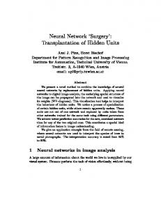
MATERIALS AND METHODS A general methodology for image classification is illustrated in figure 1. In the first step, images of the various leaf classes to be classified are acquired using an analog CCD camera interfaced with a frame grabber board. In the second phase, image preprocessing is completed. Typically, images

TRANSACTIONS OF THE ASAE

obtained during phase 1 are not suitable for classification due to factors such as noise, lighting variations, etc. These images are typically preprocessed using filters to remove unwanted features in the images. Edge detection is used in phase 3 to discover the actual boundary of the leaf in the image. Feature extraction is then executed based on specific properties among pixels in the image or their texture. After this step, statistical analysis tasks are executed to choose the best features that represent the given image, thus minimizing feature redundancy. Finally, image classification is conducted using the various detection algorithms. LEAF SAMPLE COLLECTION The leaf samples that were used in this research were collected from a single grapefruit grove (Duncan variety) in central Florida. Four different classes of citrus leaves were selected for this study. The diseased leaf samples investigated were greasy spot (Mycosphaerella citri), melanose (Diaporthe citri), scab (Elsinoe fawsettii), and normal citrus leaf. The leaf samples were collected in late spring from a number of different grapefruit trees that exhibited the various disease conditions. The degree of disease damage varied significantly between leaf samples. An attempt was made to select leaf samples that had a visibly discernable level of disease manifested. However, the degree of disease was not controlled or measured. Leaf samples were clipped with leaf stems intact and then sealed in Ziploc bags to maintain the moisture level of the leaves. Forty samples of each of the four classes of leaves were collected. The samples were brought to a laboratory and were lightly rinsed to remove any non-uniform distribution of dust. This would provide similar surface conditions for all classes of leaves. The leaf samples were then sealed in new bags with appropriate labels, and put in environmental control chambers maintained at 4°C. The leaf samples were then taken to the imaging station, and im− Image acquisition

Image processing

Edge detection

Feature extraction

Statistical analysis

Image classification Figure 1. Classification procedure of a general vision-based detection algorithm.

Vol. 48(5): 2007−2014

ages of both the front and back of the leaf samples were acquired. Preliminary investigations had demonstrated that leaf fronts and backs had different color texture features, and could be classified independently using the SAS statistical classifier DISCRIM. This implies that the classifier will have to first discriminate between leaf fronts and leaf backs, and then employ the appropriate disease classifier to discriminate between disease types. This should be a straightforward twolevel discrimination problem. It was therefore decided, for this study, to focus on identifying an appropriate classifier for leaf backs. Forty images were collected from the backs of each leaf class and stored in uncompressed JPEG format. The 40 images in each class were divided into two equal data sets, 20 samples for training and 20 samples for testing, to ensure that both the training and testing phases were representative of the population of diseased leaves found in the grove under study. An alternating image selection process was employed for the two sets, which would minimize any bias that might be introduced by the ordering of the leaves during the image capture phase. IMAGE ACQUISITION AND FEATURE EXTRACTION The 3 CCD camera (JAI, MV90) used for image acquisition was calibrated under the artificial light source using a calibration gray-card. An RGB digital image was taken of the gray-card, and each color channel was evaluated using histograms, mean, and standard deviation statistics. Red and green channel gains were adjusted until the gray-card images had similar means in R, G, and B, equal to approximately 128, which is mid-range for a scale from 0 to 255. The standard deviation of calibrated pixel values was approximately 5.0. The image acquisition system, shown in figure 2, consisted of the following principal components: S Four 16 W cool white fluorescent bulbs (4500K) with natural light filters and reflectors were located approximately 75 cm above the image plane. S The JAI MV90, 3 CCD color camera with 28-90 mm zoom lens. S A Coreco PC-RGB 24-bit color frame grabber with 480 × 640 pixel resolution, with an approximately 7 × 10 cm field of view. S MV Tools image capture software. It was decided for initial experiments that images would be acquired indoors simulating an outdoor environment. This would minimize the detrimental effects of variation in ambient lighting conditions. To simulate outdoor conditions, four 16 W cool white fluorescent bulbs (4500K) with natural light filters and reflectors were used. The spectral content of the cool white bulbs with natural light filters emulates that of natural sunlight. The camera used for image acquisition was a JAI MV90 3 CCD color camera with a 28-90 mm zoom lens. The camera was interfaced with the CPU, using a frame grabber, which converted the analog signals from the camera into digital RGB images. A Coreco PC-RGB 24-bit color frame grabber with a 480 × 640 pixel image size was chosen for this project. The field of view was approximately 9 × 12 cm. A detailed illustration of the image acquisition and classification process is given in figure 3. Algorithms for image segmentation and texture feature generation were developed in Matlab.

2009

Model 1B 2B 3B 4B [a]

Figure 2. Image acquisition system.

In the initial step, the RGB images of all the leaf samples were obtained. For each image in the data set, the following steps were repeated. Edge detection of the leaf was completed on each image of the leaf sample using Canny’s edge detector. Once the edge was detected, the image was scanned from left to right for each row in the pixel map, and the area outside the leaf was zeroed to remove any background noise. In the next step, the image size was reduced from 480 × 640 pixel resolution to 240 × 320 pixel resolution. The reduced images were then converted from 8 bits per channel RGB format to 6 bits per channel HSI format. The SGDMs (spatial gray-level dependency matrices) were then generated for each color pixel map of the image, one each for hue, saturation, and intensity. The SGDM is a measure of the probability that a given pixel at a particular gray level will occur at a distinct distance and orientation angle from another pixel, given that the pixel has a second particular gray level. It was decided during preliminary testing that the experiment would use one CCM comparison angle and one offset distance. The zero degree angle of rotation was arbitrarily selected, and an offset distance of one pixel was selected. From the SGDM matrices, the 39 CCM texture statistics described by Shearer and Holmes (1990) were generated for each image using the three-color feature co-occurrence matrices. Each SGDM matrices provided 13 texture features, resulting in a total of 39 features per image. A list of the texture statistics is given in table 1. A more complete description of this technique can be found in Haralick and Shanmugam (1974) and Shearer and Holmes (1990). RGB image acquisition (480 x 640, 8−bit)

Leaf edge detection

RGB to HIS translation (8−bit to 6−bit)

Table 1. Classification models reduced by stepwise discriminant analysis (SAS STEPDISC). Leaf Side Color STEPDISC Variable Sets[a] Back Back Back Back

HS I HSI HSI

S5, S2, H7, S6, S9, H8, H11, S12, H1, H12 I2, I13, I8, I7, I6, I3 I2, S5, I10, H11, S1, I13, S13 All variables

Stepwise discrimination variable list determined using a test significance level of 0.0001 for both the SLS (test for variable to stay) and the SLE (test to enter) variables. The texture variables listed are coded so that variables prefixed by “H” correspond to hue CCM statistics, “S” corresponds to saturation CCM statistics, and “I” corresponds to intensity CCM statistics. The number indicates the texture statistic, as follows: (1) uniformity, (2) mean intensity, (3) variance, (4) correlation, (5) product moment, (6) inverse difference, (7) entropy, (8) sum entropy, (9) difference entropy, (10) information correlation measure #1, (11) information correlation measure #2, (12) contrast, and (13) modus.

STATISTICAL ANALYSIS Once the texture statistics were generated for each image, SAS statistical analyses were conducted using the STEPDISC procedure to reduce redundancy in the texture feature set. SAS offers procedures for reducing variable set size and for discriminating between classes (SAS, 1985). STEPDISC is used to reduce the number of texture features by a stepwise selection process, which begins with no variables in the classification model. At each step of the process, the variable within the model that contributes least to the model, as determined by the Wilks’ lambda method, is removed from the model (SAS, 1985). The variable outside the model that contributes most to the model and passes the test to be admitted is added. When no more steps can be taken, the number of variables in the model is reduced to its final form. Based on these analyses, several data models were created, which are shown in table 1. In the classification process, only data models from image sets of the back sides of the leaves were used. As shown in table 1, four data models were generated for evaluation by the classifiers. Model 1B consisted of a reduced set of hue and saturation texture features, model 2B consisted of a reduced set of intensity features, model 3B consisted of a reduced set of hue, saturation, and intensity features, and model 4B consisted of all 33 HSI texture features. Input Data Preparation Once the texture feature extraction was complete, training and test data files were obtained, each containing all 39 texture features for each image. The files had 80 rows each, representing 20 samples from each of the four classes of leaves, as discussed earlier. Each row had 39 columns representing the 39 texture features extracted for a particular sample image. Each row had a Background noise zeroed

SGDM matrix generation for hue, saturation, and intensity

Image pixel reduction (to 240 x 320)

Texture statistics

Figure 3. Image acquisition and classification flowchart.

2010

TRANSACTIONS OF THE ASAE

unique number (1, 2, 3, or 4) representing the class to which the particular row of data belonged: 1 = greasy spot infected leaf, 2 = melanose infected leaf, 3 = normal leaf, and 4 = scab infected leaf. The training and test files for each of the models mentioned in table 1 were obtained by selecting only the texture features needed in that particular model from the total 39 texture features in the original data files. CLASSIFICATION USING SQUARED MAHALANOBIS DISTANCE The Mahalanobis distance is a very useful way of determining the “similarity” of a set of values from an “unknown” sample to a set of values measured from a collection of “known” samples. The actual mathematics of the Mahalanobis distance calculation has been known for some time. In fact, this method has been applied successfully for spectral discrimination in a number of cases. One of the main reasons the Mahalanobis distance method is used is because it is very sensitive to inter-variable changes in the training data. In addition, since the Mahalanobis distance is measured in terms of standard deviations from the mean of the training samples, the reported matching values give a statistical measure of how well the spectrum of the unknown sample matches (or does not match) the original training spectra. This method belongs to the class of supervised classification algorithms. Since this research is a feasibility study on whether such techniques give accurate results, supervised classification is an acceptable approach to test the efficacy of the method. The underlying distribution for the entire training data set, consisting of the four classes of leaves, was a mixed Gaussian model. Earlier research by Shearer (1986) had shown that plant canopy texture features can be represented by a multi-variate normal distribution. Each of the 39 texture features represented a normal Gaussian distribution. Thus, the feature space can be approximated to be a mixed Gaussian model containing a combination of 39 univariate normal distributions, if all the features are considered. For other models (having a reduced number of features), the feature space is a mixture of Gaussian models containing a combination of N univariate normal distributions, where N is the number of texture features in the model. Once it is known that the feature space of various classes of leaves is a mixed Gaussian model, the next step is to calculate the statistics representing those classes. Four parameter sets X [(m, S)](mean and covariance), representing the four classes of diseased and normal leaves (greasy spot, melanose, normal, and scab) were calculated using the training images. This stage represented the training phase, wherein the necessary statistical features representing various classes of leaves were calculated. After the training parameter sets were obtained, the classifier was evaluated using the test images for each class. This Input layer

Hidden layer W1ij

Bias (1)

constitutes the validation phase. The classifier was based on the squared Mahalanobis distance from the feature vector representing the test image to the parameter sets of the various classes. It used the nearest neighbor principle. The formula for calculating the squared Mahalanobis distance metric (r) is: r 2 = ( x − µ)T ∑ −1 ( x − µ)

where x = N-dimensional test feature vector (N is the number of features considered) m = N-dimensional mean vector for a particular class of leaves S = N × N dimensional covariance matrix for a particular class of leaves. During the testing phase, the squared Mahalanobis distance, for a particular test vector representing a leaf, is calculated for all the classes of leaves. The test image is then classified using the minimum distance principle. The test image is classified as belonging to a particular class to which its squared Mahalanobis distance is minimum among the calculated distances. CLASSIFICATION USING NEURAL NETWORK BASED ON BACK-PROPAGATION ALGORITHM The back-propagation network used in this analysis was a four-layer network, as shown in figure 4. The neural network toolbox in Matlab was used to construct and train the back-propagation network used in these tests. Classification tests were conducted to evaluate the performance of the neural network for classifying citrus diseases. Preliminary experiments were conducted to find a suitable network architecture. After some effort, it was determined that two hidden layers network with 10 neurons per layer performed significantly better than any other option. The architecture of the network used in this study is shown in figure 4. The output layer of the network had four neurons, one representing each disease condition. The output neuron exhibiting the strongest response was selected in the “winner take all” output scheme. The number of input layer neurons (n) matched the number of texture features in the selected data model. The transfer function used at the hidden layers and the output layer was a “tansig” function in Matlab. After importing the training dataset and the test dataset into the Matlab workspace, a network was constructed using the command “newff,” which is inherent in the Matlab neural network toolbox. Then the network was trained using the function “train.” The test data was simulated using the function “sim.” The Matlab technical literature gave the following explanation for the function “newff.” The function “newff” creates a feed-forward back-propagation network. The syntax for the function is as follows: Hidden layer

W2ij

Bias (2)

(1)

Output layer Wjk

Bias (3)

Figure 4. Network used in feed-forward back-propagation algorithm.

Vol. 48(5): 2007−2014

2011

Input layer

Radial basis layer

Linear output layer

wij

wij

Bias (1)

Bias (2) 2 neuron

80 neuron Figure 5. Neural network based on radial basis function used in leaf classification.

net = newff (PR, [S1, S2,..., SNl], {TF1, TF2,..., TFNl}, BTF, BLF, PF)

(2)

where PR = R × 2 matrix of minimum and maximum values for R input elements Si = size of the ith layer, for Nl layers TFi = transfer function of the ith layer, default = “tansig” BTF = back-propagation network training function, de fault = “trainlm” BLF = back-propagation weight/bias learning function, default = “learngdm” PF = performance function, default = “mse.” The above command returns an N-layer feed-forward back-propagation network. The parameters used in the feed-forward back-propagation network were “trainlm,” which designates the Levenberg-Marquardt training optimization; “learngdm,” which designates the gradient descent with momentum learning function; mean square error (MSE) performance function; and 3000 epochs. The MSE goal was 0.0000001. Consequently, the network would train until either the epochs expired or the MSE goal was achieved. With these parameters and the training dataset, the network was trained. Once training was complete, the network was tested using the test data for each class of leaves. The performance of the neural network classifier was recorded. CLASSIFICATION USING NEURAL NETWORK BASED ON RADIAL BASIS FUNCTIONS The Neural Network toolbox of Matlab was used to conduct the classification test on radial basis functions. The Neural Network toolbox GUI interface was used to create and test the radial basis network. The network used for this analysis is shown in figure 5. The network used 80 basis functions, as can be seen in figure 5. This is obvious because the input had 80 total input vectors for training. The output is an encoded 2 × 1-column vector: greasy spot = [0 0], normal = [1 0], melanose = [0 1], and scab = [1 1]. In this analysis, the ideal target output vectors used for training for various classes of leaves are as follows: the outputs of the radial basis function are fuzzy

Model 1B 2B 3B 4B

2012

Table 2. Classification results for SAS generalized square distance classifier in percent correct. Color Greasy Feature Spot Melanose Normal Scab Overall HS I HSI ALL

100 100 100 100

100 100 100 100

90 95 100 100

95 100 100 100

96.3 98.8 100 100

outputs giving a measure of strength; the level of fuzziness was determined by any value 0.5 being equivalent to 1; the parameters used in building this network were radial basis function (exact fit) and a spread constant of 629.2455. The data models described in table 1 were evaluated as discussed earlier. The input was normalized before being fed into the network. After the network was built, test data for each class were fed to the network and the classification task was completed based on the target vectors and fuzzy criterion described above.

RESULTS The results shown in table 2 were obtained using a generalized square distance classifier in SAS. The results were part of preliminary investigations, which used a non-real time classification approach. The results found during this study provide a benchmark for comparing real-time classification approaches, since the classification results were nearly perfect. The results reported better classification accuracies for all the data models. In particular, models 3B and 4B achieved perfect overall classification rates. Model 1B achieved an overall accuracy of 96.3 %, and model 2B achieved an accuracy of 98.8%. The results shown in table 3 were obtained using the Mahalanobis minimum distance classifier. In particular, models 1B and 2B achieved better overall classification rates. Model 1B achieved an overall accuracy of 98.75 %, and model 2B achieved an accuracy of 97.5%. Therefore, model 1B is the overall best model using this classifier. It was also observed that one model (model 3B) was unable to discriminate greasy spot from the other classes, incorrectly classifying all greasy spot images. The source of this anomaly is unknown, but it occurs again in one of the neural network models. Obviously, in this case, the reduced HSI features selected by STEPDISC were inappropriate for the Mahalanobis classifier. The results from the two statistical classifiers demonstrate that such techniques can be used for disease leaf classification. In general, tables 2 and 3 show close agreement between

Model 1B 2B 3B 4B

Table 3. Classification results for Mahalanobis distance classifier in percent correct. Color Greasy Feature Spot Melanose Normal Scab HS I HSI ALL

100 100 0 90

100 95 100 100

100 95 100 80

95 100 100 60

Overall 98.75 97.5 75 85

TRANSACTIONS OF THE ASAE

Model 1B 2B 3B 4B

Table 4. Classification results for back-propagation neural network in percent correct. Color Greasy Feature Spot Melanose Normal Scab Overall HS I HSI ALL

100 95 100 100

90 95 90 95

95 15 95 100

95 100 95 100

95 76.25 95 98.75

the two classifiers for models 1B and 2B. Although model 2B, which relies on intensity features, performed well in both cases, it may have limited usefulness in outdoor applications due to inherent intensity variations in outdoor lighting conditions. Hence, model 1B, which relies on hue and saturation features, emerges as the best model in classifiers based on statistical classification. The results shown in table 4 were obtained using a back-propagation neural network. In particular, models 1B, 3B, and 4B achieved excellent overall classification rates. Models 1B and 3B achieved an overall accuracy of 95%, and model 4B achieved an accuracy of 98.75%. Model 1B emerges as the better model than 3B and 4B, since it does not rely on intensity features and has significantly less computational requirements. The results shown in table 5 were obtained using a neural network based on radial basis functions. In particular, models 1B, 3B, and 4B achieved better overall classification rates. Models 1B and 3B achieved an overall accuracy of 86.25%, and model 4B achieved an accuracy of 97.5%. The analyses for neural network classifiers proved that model 4B achieved better classification accuracies in both cases. This was logical, since model 4B consists of more texture features, which are beneficial in neural network applications. However, in a real-world application, model 4B may be disadvantageous due to the large processing time required for calculating all texture features, and due to variance in ambient lighting conditions. From the simulation results, it was concluded that model 1B, consisting of features from hue and saturation, was the superior classification model for classifying diseased citrus leaves when using the two neural networks. Elimination of intensity texture features is a major advantage, since it may minimize the effect of lighting variations in an outdoor environment. In addition, the algorithm would be faster due to the elimination of the intensity CCM calculation and fewer texture features would be required than with model 4B (10 versus 39).

SUMMARY AND CONCLUSIONS A study was completed to investigate the use of computer vision for classifying citrus leaf diseases. Four different classes of citrus leaves (greasy spot, melanose, normal, and

Model 1B 2B 3B 4B

Table 5. Classification results for radial basis neural network in percent correct. Color Greasy Feature Spot Melanose Normal Scab HS I HSI ALL

Vol. 48(5): 2007−2014

100 100 95 100

100 20 80 95

85 75 85 100

60 0 85 95

Overall 86.25 48.75 86.25 97.5

scab) were used for this study. Image processing algorithms were developed for feature extraction and classification. The feature extraction process used color co-occurrence (CCM) methodology, which uses both the color and texture of an image to arrive at unique features that represent the image. SAS discriminant analysis was used to reduce the variable sets and to evaluate the potential classification accuracies, which could be achieved using a traditional statistical classifier. SAS discriminant analysis achieved classification accuracies above 96% on all data models, with the strongest models achieving 100% accuracies. This provided a benchmark for comparison with other classifiers more appropriate for real-time applications. Classification tests were conducted on three alternate classification algorithms: a statistical classifier using the Mahalanobis minimum distance method achieved overall classification accuracies as high as 98%, a neural network classifier using the back-propagation algorithm achieved overall accuracies as high as 98%, and a neural network classifier using radial basis functions achieved overall accuracies as high as 96%. An image texture feature data set, which used a reduced hue and saturation feature set (model 1B), emerged as the best data model for the task of citrus leaf classification. This was due to its reduced number of data variables, which would minimize computation time, and the elimination of intensity features, which may prove beneficial in highly variable outdoor lighting conditions. The Mahalanobis statistical classifiers gave the best results for model 1B, with an overall accuracy above 98%, while the back-propagation neural network achieved a 95% overall accuracy. The analyses proved that such methods could indeed be used for classifying diseased citrus leaves under controlled laboratory lighting conditions. Consequently, it is recommended that both the Mahalanobis statistical classifier and the back-propagation neural network classifier be further considered when applying the texture-based features in an outdoor scene, which will be the focus of future studies. ACKNOWLEDGMENTS This research was conducted at the University of Florida, Institute of Food and Agricultural Sciences, through funding provided through the USDA-IFAFS.

REFERENCES Burks, T. F., S. A. Shearer, and F. A. Payne. 2000. Classification of weed species using color texture features and discriminant analysis. Trans. ASAE 43(2): 441-448. Crowe, T. G., and M. J. Delwiche. 1996. Real-time defect detection in fruit: Part II. An algorithm and performance of a prototype system. Trans. ASAE 39(6): 2309-2317. Edwards, J., G. Sweet, and C. Haven. 1986. Citrus blight assessment using a microcomputer; quantifying damage using an apple computer to solve reflectance spectra of entire trees. Florida Scientist 49(1): 48-53. Haralick, R. M., and K. Shanmugam. 1974. Combined spectral and spatial processing of ERTS imagery data. Remote Sensing of Environ. 3(1): 3-13. Miller, W. M., J. A. Throop, and B. L. Upchurch. 1998. Pattern recognition models for spectral reflectance evaluation of apple blemishes. Postharvest Biology and Tech. 14(1): 11-20. Nakano, K. 1997. Application of neural networks to the color grading of apples. Computers and Electronics in Agric. 18(2-3): 105-116.

2013

Pinter, P. J., J. L. Hatfield, J. S. Schepers, E. M. Barnes, M. S. Moran, C. S. T. Daughtry, and D. R. Upchurch. 2003. Remote sensing for crop management. Photogrammetric Eng. and Remote Sensing 69(6): 647-664. SAS. 1985. Statistics. In SAS User’s Guide. 5th ed. Cary, N.C.: SAS Institute, Inc. Shearer, S. A. 1986. Plant identification using color co-occurrence matrices dervived from digitized images. PhD diss. Columbus, Ohio: Ohio State University.

2014

Shearer, S. A., and R. G. Holmes. 1990. Plant identification using color co-occurrence matrices. Trans. ASAE 33(6): 2037-2044. Sudbrink Jr, D. L, A. F. Harris, and J. T. Robbins. 2000. Remote sensing of late-season pest damage to cotton and wild host plants of tarnished plant bug in the Mississippi delta. In Proc. Beltwide Cotton Conference, 2: 1220-1223. Memphis, Tenn.: National Cotton Council. Yang, C., S. Prasher, and J. Landry. 1998. Application of artificial neural networks to image recognition in precision farming. ASAE Paper No. 983039. St. Joseph, Mich.: ASAE.

TRANSACTIONS OF THE ASAE