Exact algorithms for a generalization of the order ... - CiteSeerX

Exact algorithms for a generalization of the order acceptance and scheduling problem in a single-machine environment Fabrice Talla Nobibon and Roel Leus∗ Research group ORSTAT Faculty of Business and Economics, K.U.Leuven Naamsestraat 69, B-3000 Leuven, Belgium {Fabrice.TallaNobibon ; Roel.Leus}@econ.kuleuven.be

Abstract: This paper studies a generalization of the order acceptance and scheduling problem in a single-machine environment where a pool consisting of firm planned orders as well as potential orders is available from which an over-demanded company can select. The capacity available for processing the accepted orders is limited and each order is characterized by a known processing time, delivery date, revenue and a weight representing a penalty per unit-time delay beyond the delivery date. We prove that the existence of a constant-factor approximation algorithm for this problem is unlikely. We propose two linear formulations that are solved using an IP solver and we devise two exact branch-and-bound procedures able to solve instances with up to 50 jobs within reasonable CPU times. We compare the efficiency and quality of the results obtained using the different solution approaches. Keywords: order acceptance, scheduling, single machine, integer programming, branchand-bound, firm planned orders.

1

Introduction

Many organizations give no formal consideration to either order acceptance or rejection. Instead, an order-entry process is operated that tacitly accepts all orders. In today’s competitive manufacturing environment, an organization must respect order deadlines agreed to with customers, but order acceptance often takes place without consideration of the effect on the planning of the other jobs in the order portfolio. Herbots et al. [14] observe that “this is often the consequence of the functional separation between the order acceptance decision, which is made by the sales department, and the capacity planning, which usually lies in the hands of the production department”. The sales department tends to accept as many jobs as possible while the production department attempts to meet the promised delivery dates. In order to avoid conflict of interest between these two departments, which may result in considerable delays, violated due dates and/or excessive use of highly expensive non-regular capacity, an integration of job selection and planning is needed [12, 14, 37]. Over the past decade, order acceptance has gained increasing attention both from academia as well as from practitioners communities. As clearly described by Rom and Slotnick [27], “this decision is intricate because it should strike a balance between the revenue obtained from an accepted order on the one hand, and the (opportunity) costs of capacity as well as potential tardiness penalties on the other hand”. This paper studies ∗

Corresponding author. Tel +32 16 32 69 67. Fax +32 16 32 66 24.

1

a generalization of the order acceptance and sequencing problem. Order acceptance refers to the selection decision an over-demanded company has to make, while sequencing determines the order in which accepted jobs are executed. More specifically, the focus of this paper is on the order acceptance and sequencing decisions of an organization that has a pool consisting of firm planned orders as well as potential orders to choose from, while orders have known processing times, delivery dates and revenues. The capacity available for processing the accepted orders is limited. In addition, the urgency of individual orders may be emphasized by the importance of the client and/or the contract details. In this article, we examine a generalization of the order acceptance and planning problem on a specialized scarce resource, which is represented as a single machine and which constitutes the bottleneck of the manufacturing environment. We propose two linear formulations and devise two exact branch-and-bound algorithms to solve the problem of deciding which potential orders to retain and which to reject for profit maximization, and we determine the processing order of the accepted jobs. By means of computational experiments on a number of benchmark datasets, we solve instances with up to 50 jobs. The problem studied can be seen as a generalization of two existing problems. The first problem is the order acceptance and sequencing problem with weighted-tardiness penalties studied by Slotnick and Morton [31]. Our problem reduces to the latter one when the pool of firm planned orders is empty and all jobs are eligible for rejection. The second problem is the total-weighted-tardiness scheduling problem studied by Potts and Van Wassenhove [25], Pan and Shi [24] and Tanaka et al. [33], among others. It corresponds with our problem when all orders are firm planned orders. The contributions of this article are the following: we provide the first description and study of this generalized order acceptance and sequencing problem, which builds a bridge between two existing problems, namely single-machine scheduling with weightedtardiness objective and job selection and sequencing with weighted-tardiness penalties. We prove the non-approximability of the problem and propose two mixed-integer linear formulations, which can be solved using an IP solver. We also develop two exact branchand-bound algorithms that are able to solve instances with up to 50 jobs in less than two hours. The remainder of this article is structured as follows. First, we survey the existing literature in Section 2. In Section 3, we provide a formal description of the problem that we wish to solve. Section 4 contains the proof of the non-approximability result and the two linear formulations. Section 5 is devoted to the development of two branch-and-bound algorithms. We comment the results of the computational experiments in Section 6 and conclude in Section 7.

2

Literature review

Excellent literature surveys on the topic of order acceptance and scheduling are provided by Rom and Slotnick [27], Guerrero and Kern [12], Keskinocak and Tayur [16] and Roundy et al. [28]. The objective of this section is therefore not to provide an exhaustive listing of the existing literature, but rather to survey the different perspectives that have been developed on the topic by different researchers, with a particular focus on the work in single-machine environments. Although the total-weighted-tardiness problem is

2

strongly NP-hard [18, 19], Potts and Van Wassenhove [25] have developed a branch-andbound algorithm that efficiently solves problems with up to 50 jobs; recently, Pan and Shi [24] have derived a new bound that allows this algorithm to solve instances with up to 100 jobs and Tanaka et al. [33] have presented a Successive Sublimation DynamicProgramming (SSDP) method able to solve instances with up to 300 jobs. This review will therefore only discuss the most closely related articles on the subject of order acceptance and scheduling. First, we discuss the order acceptance problem with weighted-tardiness penalties; subsequently, we briefly consider alternative objective functions and on-line decision making. Slotnick and Morton study the single-machine job selection and sequencing problem with deterministic job processing times and job rewards; their objective is to maximize the rewards in case of lateness [30] and tardiness [31] penalties. A pseudo-polynomialtime algorithm to solve the former problem was developed by Ghosh [10]. The problem was extended in [20] to multiple periods for the case where rejecting a job will result in the loss of all future jobs from that customer. An exact approach for solving the order acceptance problem with weighted-tardiness penalties was developed in [31]. Since the proposed algorithm can only deal with very moderately sized problem instances (at most ten jobs), suboptimal algorithms were also presented. Other heuristics include genetic algorithms [27] and greedy algorithms [2]. Yang and Geunes [35] consider an extension of the problem where job processing times are reducible at a cost and every job has a release time. In their paper, Yang and Geunes develop an optimal algorithm for maximizing schedule profit for a given sequence of jobs, along with heuristics to solve the entire problem. Sengupta [29] studies a similar problem with maximum lateness and tardiness objectives, and proposes pseudo-polynomial-time algorithms and approximations schemes. Both a mixed-integer programming (MIP) formulation as well as a branchand-bound algorithm for solving the order acceptance problem with weighted-tardiness penalties are mentioned in the very brief article of Yugma [36]; he reports (without details) results “in reasonable time” via MIP for up to 15 jobs, and up to 30 using branch-and-bound. Finally, Oguz et al. [23] look into a generalization of the order acceptance problem with weighted-tardiness penalties that includes release times, deadlines and sequence-dependent setup times; they conclude that a MIP-solution is not attainable for problem sizes exceeding 15 jobs and resort to a constructive heuristic and an iterative improvement heuristic that is based on simulated annealing. For the same problem, Cesaret et al. [4] find higher-quality solutions by means of tabu search. Other objective functions for the selection and sequencing problem have been considered in literature. Engels et al. [8] seek to minimize the sum of the weighted completion times of the scheduled jobs and the total rejection penalty of the rejected jobs. A related objective function is used in [21] for the unbounded parallel-batch-machine scheduling problem with release dates. A parallel batch machine can process a number of jobs simultaneously, so that the makespan is the same for all jobs in a batch. A different but related problem is the job-interval selection problem (JISP), where a job is determined by a set of intervals. In [5], some special cases of the JISP are considered. The paper develops algorithms that aim to maximize the number of jobs scheduled between their release dates and deadlines. Another objective function was examined by Gupta et al. [13], who develop an efficient polynomial-time dynamic-programming method that solves the project selection and sequencing problem (a fixed number of projects is selected from a 3

set) while maximizing the net present value of the total return. De et al. [6] study the sequencing problem and minimize the weighted number of tardy jobs. In [6], a projectdependent cost is charged when starting the execution of a project, leading to a selection problem. It is also assumed that a revenue is collected at the completion of a project. The goal is to maximize the expected rewards of a selection of jobs with random processing times and random deadlines. Meng-G´erard et al. [22] study a related problem with unit durations inspired by a practical case of a satellite launcher, and describe polynomial-time dynamic-programming recursions for some special cases. The on-line problem, in which projects arrive dynamically over time and need to be selected or rejected upon arrival, has been studied by several authors for a broad range of objective functions. For dynamic arrivals with a single resource constraint, Kleywegt and Papastavrou [17] study a dynamic and stochastic knapsack problem, where the size of the knapsack represents the available resource quantity. Each arrival demands some amount of the resource, and a reward (unknown prior to the job arrival) is received upon acceptance. They provide an optimal acceptance policy that maximizes expected profits. For the batch process industry, Iv˘anescu et al. [15] develop policies that focus on delivery reliability while maintaining high utilization rates. Epstein et al. [9] consider a single-machine on-line job selection and scheduling problem with job-dependent rejection penalties. Their algorithm aims to minimize the total completion time of accepted jobs plus job rejection penalties.

3

Problem statement

A set of jobs N = {1, 2, . . . , n} with durations pi (i ∈ N ) is to be scheduled on a single machine; all jobs are available for processing at the beginning of the planning period. Each job i has a due date di and a revenue Qi ; the weight wi represents a penalty per unit-time delay beyond di in the delivery to the customer. The pool N of jobs consists of two disjoint subsets F and F¯ (N = F ∪ F¯ and F ∩ F¯ = ∅), for which F comprises the firm planned orders and its complement F¯ contains the ‘optional’ jobs (the ones that can still be rejected). Our objective is to maximize total net profit, that is, the sum of the revenues of the selected jobs minus applicable total-weighted-tardiness penalties incurred for those jobs. There are two decisions to be made: which jobs in F¯ to accept, and in which order to process the selected subset. We call M the set of jobs selected for processing, so F ⊆ M ⊆ N . If we let m = |M |, the sequencing decisions can be represented by a bijection π : {1, 2, . . . , m} 7→ M , where π(t) is the job in position t in the sequence. Each such bijection is in one-to-one correspondence with a total order on set M . The objective is thus m X max Qπ(t) − wπ(t) (Cπ(t) − dπ(t) )+ , (1) M,π

t=1

P −1 where Ci is the completion time of job i, i.e. Ci = πt=1 (i) pπ(t) , and s+ = max{s, 0}. In the remainder of this text, we refer to (1) as either the objective function or the problem formulation; there will be little danger of confusion. When N = F , all jobs are mandatory and the P problem reduces to the single-machine total-weighted-tardiness scheduling problem 1|| wi Ti [24, 25, 33]. When N = F¯ , on the 4

other hand, the problem is equivalent to the order acceptance problem with weightedtardiness penalties discussed in [27, 31], which is akin to a number of other recently examined optimization problems, as discussed in the literature review. This problem contains the scheduling problem; it is therefore strongly NP-hard. The branch-and-bound procedure in [31] only solves relatively small problem instances (at most ten jobs) and is primarily used as a benchmark for evaluating the performance of heuristics.

4

Non-approximability and linear formulations

In this section, we first show that it is unlikely that a constant-factor approximation algorithm can be developed for solving the problem (1); subsequently, we present two mixed-integer linear formulations of (1), which can be solved using an IP solver.

4.1

Non-approximability

The next result shows that (1) is difficult to solve even approximately. We prove this non-approximability result by showing that any polynomial-time constant-factor approximation algorithm for solving (1) can be used to solve the following variant of Partition: INSTANCE: A finite set A = {1, 2, . . . , 2q} P (where q is an integer greater than 0) with 1 + size s(i) ∈ Z for each i ∈ A, and K = 2 i∈A s(i). P QUESTION: Does there exist a subset A0 ⊂ A with |A0 | = q and i∈A0 s(i) = K? By adding |A| dummy elements of size 0 to an instance of the usual Partition problem, one easily sees that this variant of Partition is as hard as the original problem. Proposition 1. Unless P = N P , there is no polynomial-time algorithm that guarantees a constant-factor approximation for solving the problem (1). Proof: For a given arbitrary instance of Partition, consider the following polynomial reduction to an instance of (1) with n = 2q + 2 jobs. The set of firm planned orders F = {2q + 1, 2q + 2} and we let δ = 2K + 1. The properties of each job are the following: for job i = 1, . . . , 2q we have a revenue Qi = δs(i), the processing time pi = δ + s(i), the due date di = qδ + K + 2 and the weight wi = s(i)(δ + 1). For the last two jobs, we have Q2q+1 = Q2q+2 = δ, p2q+1 = p2q+2 = 1, d2q+1 = d2q+2 = 1 and w2q+1 = w2q+2 = δ(K + 2). We prove that by solving this instance of (1) with a constantfactor approximation algorithm, we can infer the answer to the Partition instance. If the instance of Partition is a YES instance then an appropriate set A0 exists. We consider the solution of our problem that selects the jobs in A0 (jobs built from the elements in A0 ) plus those in F and executes them as follows. Job 2q + 1 is first, job 2q + 2 second and the jobs in A0 in any order thereafter. For this solution, the only job delivered after its due date is job 2q + 2. The total revenue obtained from selected jobs is Kδ for jobs built from the elements in A0 plus 2δ received for job 2q + 1 and job 2q + 2. The latter job, however, is tardy by one time unit, for which we incur a cost δ(K + 2). Together, the objective value of this solution is Kδ +2δ −δ(K +2) = 0, which can be seen to be the highest value possible for any feasible solution. Therefore, a constant-factor 5

approximation algorithm will provide an optimal solution, from which we can easily infer the elements of A0 . Conversely, if a constant-factor approximation algorithm leads to an objective value different from 0, we conclude that the instance of Partition is a NO instance.  Proposition 1 implies that while heuristics can be devised to produce solutions to large instances of our problem, there is no guarantee that they will always attain at least a specific proportion of the optimal objective value.

4.2

Linear formulations

We present an assignment formulation and a time-indexed formulation of our problem, which can be solved using an IP solver. 4.2.1

Assignment formulation

This formulation uses binary decision variables yi ∈ {0, 1} (i ∈ N ), which take the value 1 if job i is accepted and 0 otherwise, and binary variables xit ∈ {0, 1} (i ∈ N , t ∈ {1, . . . , n}) for identifying the position of the accepted jobs in the sequence of execution: the variable xit is equal to 1 if job i is accepted and is the tth job processed, and to 0 otherwise. We also introduce the binary variables zji ∈ {0, 1} (i, j ∈ N , i 6= j), which are equal to 1 if and only if both jobs i and j are accepted and job j is executed before job i. To complete our formulation, we need real variables Ti ≥ 0 representing the tardiness of the jobs i ∈ N . We propose the following mixed-integer linear formulation ASF: (ASF)

max

n X

(Qi yi − wi Ti )

(2)

i=1

s.t.

yi = 1 n X xit yi =

∀i ∈ F,

(3)

∀i ∈ N,

(4)

t = 1, . . . , n,

(5)

i, j ∈ N, i 6= j,

(6)

i, j ∈ N, t = 2, . . . , n, i 6= j,

(7)

i ∈ N,

(8)

t=1 n X

xit ≤ 1

i=1

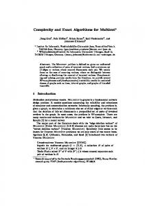
zji ≤ yi and zji ≤ yj X X xjq + xiq ≤ 1 + zji q Ju , with Ju the job added at the parent node. To illustrate this in Figure 1, consider node 3 where job 3 is added. One might expect the tree to include a child node of node 3 with selection {1, 2, 3, 4}, but because 1 < 3 this child node is not considered. Notice that the use of the above criterion may yield a strongly unbalanced branching tree and that we do not compute UBs for nodes that are certainly leaves of the tree. In Figure 1, node 3 is a leaf node because it selects job 3, the job with the highest index in R. Node 2 is a leaf node because the LB of 9 is already equal to the UBs, and the potential child node with selection {1, 2, 3, 4} is therefore not entered. 5.1.3

Node selection

We explore the branching tree in a best-first search (BFS) manner. During the search, a list of unfathomed nodes is kept in non-increasing order of their UB. The first node in the list is the next node to investigate. When a new node is created, the list is updated

10

by inserting that node at the appropriate position such that the non-increasing-UB order is preserved. 5.1.4

Scheduling algorithm and lower bound

In each node u, we have a set Mu of selected jobs, which contains the firm planned orders, that is F ⊆ Mu . Therefore, each set Mu together with any execution sequence for the jobs in Mu constitutes a feasible solution to our problem. We use the B&B algorithm developed by Potts and Van Wassenhove [25] to optimally schedule the jobs in Mu to minimize the total weighted tardiness. We note that the recent SSDP algorithm proposed by Tanaka et al. [33] represents an attractive alternative for this scheduling phase, which is not explored in P this article. The objective value of the solution obtained at node u is the total revenue i∈Mu Qi from the accepted jobs minus the tardiness costs provided by Potts and Van Wassenhove’s algorithm. This value is a LB of the optimal objective value of our problem. 5.1.5

Upper bound

At node u, an UB is computed only if node u is not a leaf node. We have implemented three UBs. The first one is obtained by solving an assignment problem; this bound generalizes a similar bound used by Slotnick and Morton [31]. The second bound is the optimal objective value of an order acceptance and scheduling problem with weightedlateness penalties and the last bound is the objective value of the LP-relaxation of TIF. Assignment bound In the computation of this UB, we relax the implicit non-preemption constraint on the jobs. Each job is divided into joblets with a duration of one time unit, and these joblets are then scheduled independently of each other. The resulting scheduling problem is solved by an assignment problem that assigns joblets to unit-duration time buckets. At node u, we include dummy joblets and dummy positions to allow for the rejection of joblets stemming from jobs not in Mu . Consider a node u at level ` of the search tree and let Ju be the last job added; it holds that u ≥ `. The set Su = N \ ({J1 , . . . , Ju−1 } \ Mu ) contains the jobs that remain eligible for selection in the descendant nodes of Pnode u (and some of them have already been selected with certainty); let K = i∈Su pi . We associate with the allocation of any joblet of a job in Mu to a time instant larger than K a very large cost in the assignment problem, while the assignment of any joblet of jobs not in Mu to a time instant larger than K and the assignment of any dummy joblet corresponds with zero cost. A non-dummy joblet assigned to a time bucket with index lower than or equal to K corresponds with acceptance of that joblet; the contribution of such a combination to the objective function is determined based on the per-joblet reward, weight and due date. The per-joblet reward and weight are obtained by dividing the original job’s reward and weight by the job’s processing time; the due date of a joblet is a function of the position of the joblet (within the job) and the job’s due date [27, 31]. The assignment problem is solved using a cost-scaling algorithm [1, 11] and the optimal value constitutes an UB.

11

Lateness bound In an arbitrary node u of the search tree, the total net profit is max

Mu ⊆M ⊆Nu ,π

|M | X

Qπ(t) − wπ(t) (Cπ(t) − dπ(t) )+ ,

t=1

where Nu = N \ {ji ∈ R : Ji < Ju and Ji ∈ / Mu }, with Ju the last job accepted. We replace the tardiness penalties by lateness penalties; jobs can then also receive a reward for being early. We obtain the following problem: max

Mu ⊆M ⊆Nu ,π

|M | X

Qπ(t) − wπ(t) (Cπ(t) − dπ(t) ).

t=1

This latter problem is a generalization of the job selection and sequencing problem with weighted-lateness penalties [10, 30]. The generalization resides in the fact that a specific subset of jobs (namely Mu ) is necessarily selected. The pseudopolynomial-time dynamic-programming algorithm proposed by Ghosh [10] is easily modified to solve this problem. The optimal objective value provides an UB for our problem. LP-relaxation bound This bound is the optimal objective value of the LP-relaxation of TIF where for each job j ∈ Mu \ F , the sense of the corresponding constraint (13) is changed into equality. It turns out that the assignment bound is virtually always at least as strong as the lateness bound, but also computationally more expensive. Similarly, the LP-relaxation bound is usually at least as strong as the assignment bound, but its computation takes more time. In the working paper [32], we investigate two combinations of the first two UBs. The first combination computes an assignment bound at the root node, while at all subsequent nodes a lateness bound is computed first. If the lateness value is less than or equal to α times the UB of its parent node (α ∈]0, 1[) then an assignment bound is computed, in an attempt to prune the node. The second combination is based on similar principles but α varies during the search, by choosing its value as the number of jobs accepted at the parent node divided by the number of jobs accepted at the child node. The use of these two combinations in the implementation of the B&B, however, did not improve the CPU time achieved by the initial upper bounds, and we will not report the computational results of these implementations in Section 6.

5.2

Direct B&B algorithm

The main steps of the direct B&B algorithm are described in this section. 5.2.1

Branching strategy

Figure 2 depicts the search tree explored by the direct B&B algorithm when applied to Example 1. Optimal solutions are found in node 9 and node 10. The root node (node 1) represents the situation where no job has been accepted yet. The LB of −2 corresponds to the value achieved by the solution that selects all the jobs in F and 12

Level 0

Level 1

LB = −2 UB2 = 9

node 1

node 2

LB = −7 UB2 = 1

Level 2

1

node 5

node 4

LB = −2 = −7 2 LB UB2 = −1 UB2 = 1 node 3

3

node 6 LB = 9 UB2 = 9

41

LB = 8 UB2 = 9

4

node 7

LB = 8 UB2 = 9

42

node 8

LB = 8 UB2 = 8

43

Level 3 LB = 9 412 UB2 = 9 node 9

LB = 9 UB2 = 9 423 node 10

Figure 2: Illustration of the direct B&B algorithm with lateness bound U B2 for solving Example 1. Inside each node, the corresponding (possibly partial) solution is represented as a sequence of job indices.

executes them in increasing order of job index. The UB reported in Figure 2 is a lateness bound; for more details, see Section 5.2.3. At level 1 of the search tree, n new nodes are created representing n (possibly partial) solutions, each generated by selecting one job and scheduling it at the first position. In Figure 2, these are node 2, which selects job 1 (whence the entry ‘1’ inside the node), node 3, which selects job 2, and similarly up to node 5. Given a parent node at level k − 1 (k ≥ 1), we create n − k + 1 child nodes each with k jobs selected with known position: the job added at level k is the k th job processed. Node 5, for instance, has three child nodes (nodes 6, 7 and 8), each of which selects one additional job to be executed immediately after job 4. At node 6, for example, job 1 is selected and the text ‘41’ in the node means that job 4 comes first, followed by job 1. In the same way as in the two-phase algorithm, the branching tree is explored in a BFS manner. 5.2.2

Lower bound

At a given node u of the branching tree, let Mu ⊆ N be the set of selected jobs and Vu the return (net profit) obtained from the selection of jobs in Mu and the sequencing decisions inherent in node u. Two cases can occur. Either (1) F ⊆ Mu , in which case Vu is a LB, or (2) F * Mu , and then Vu is not a LB at node u. In the latter case, our LB is the objective value of the solution that selects the jobs in F ∪ Mu and executes them following the sequence corresponding with node u for Mu , followed by the jobs in F \ Mu in increasing order of job index. 13

5.2.3

Upper bound

All three of the upper bounds presented in Section 5.1.5 for the two-phase algorithm only ¯ u the need minor modifications to be applicable in the direct algorithm. We denote by M complement N \ Mu . At node u, the contribution to the objective function of the jobs ¯ u needs to in Mu is known exactly; therefore, only the contribution of potential jobs in M be bounded. Because the |Mu | selected jobs are scheduled at the first P |Mu | positions, the ¯ due date of each job in Mu is updated accordingly by subtracting i∈Mu pi ; we refer to ¯ u. these new values as d¯i for i ∈ M Assignment bound This UB is similar to the one presented in [31], apart from the updated due dates. The sum of Vu and the optimal objective value of the assignment problem yields an UB. Lateness bound At node u, the unscheduled jobs can achieve a net profit of max

¯ u ,π M ⊆M

|M | X

Qπ(t) −wπ(t) (Cπ(t) −d¯π(t) )+ ≤ max

¯ u ,π M ⊆M

t=1

|M | X

Qπ(t) −wπ(t) (Cπ(t) −d¯π(t) ) = ∆,

t=1

where F \ Mu ⊆ M . The value ∆ + Vu is an UB. LP-relaxation bound At node u, the LP-relaxation of a restricted formulation TIF is ¯ u with updated due dates. The sum of the optimal solved, including only jobs in M objective value and Vu constitutes an upper bound. In addition to the two UB-combinations mentioned for the two-phase B&B, two more combinations have been investigated in [32] for the direct B&B algorithm. One computes the assignment bound at the root node, while a lateness bound is computed first at subsequent nodes. If the value of the LB at that node is less than or equal to α ∈]0, 1[ times the LB of its parent node then an assignment bound is also computed, in an attempt to prune the node. The second combination follows the same idea but puts α equal to the number of jobs accepted at the parent node divided by the number of jobs accepted at the current node. More details on these combinations and the resulting computational results can be found in [32]. 5.2.4

Dominance rules

Below, we outline some global and local dominance rules that are used as pruning devices for the direct B&B algorithm. Global dominance rules The global dominance rules presented below generalize Emmons’ rules [3, 7, 26]. The goal of these rules is to identify for each job j a set Bj containing jobs that, if selected together with job j, can be processed before job j, and Aj , a set of jobs that, if selected together with job j, can be executed after job j. Let BjF be the set of jobs in F that must be processed before job j, and AFj the set of jobs in F that must be processed after job j. Both BjF and AFj are initially empty, and the rules below are applied iteratively.

14

Lemma 1. If job i and job j are selected, then there is an optimal sequence in which job i is processed before job j, if one of thePfollowing conditions holds: Rule 1: pi ≤ pj , wi ≥ wj and di ≤ max{dj , pj + h∈B F ph }. j P Rule 2: wi ≥ wj , di ≤ dj and dj + pj ≥ h∈N \AF ph . i P Rule 3: dj ≥ h∈N \AF ph . i

Proof: The proof of these three rules follows from the proof proposed by Rinnooy Kan et al. [26]. In fact, if job i and job j are accepted then the set of selected jobs contains F ∪{i, j}. For the scheduling problem associated with that set, Rule 1 corresponds to Corollary 1 in [26], Rule 2 corresponds to Corollary 2 and Rule 3 to Corollary 3.  When F = N , these three rules are exactly Emmons’ rules [26] for the totalweighted-tardiness scheduling problem; Lemma 1 proposes similar rules for the order acceptance problem. As for the scheduling problem, these three rules are used to construct a predecessor graph. Unlike the scheduling problem, however, where each arc in the graph is unconditionally respected, in this article a precedence relation imposing the execution of job i before job j is respected only in the branches where both job i and job j are accepted. Once a number of precedence-related activity pairs have been distinguished, additional pairs can be transitively inferred. Our implementation of this transitivity is slightly different from [26] because, again, we need to select jobs as well as schedule them. We distinguish between jobs in F and those in N \ F and proceed as follows. Whenever we identify a new dominant decision of the form ‘job j precedes job k’, we consider two possible cases: Case 1: If job j ∈ F then we ensure that job k and each successor of k is processed after job j and any of its predecessors. Case 2: If job k ∈ F then we enforce that job j and each predecessor of j is executed before job k and any of its successors. Local dominance rules At each node of the branching tree, we use two local dominance rules as pruning devices. The following lemma presents the selection criterion. At node u, let Ju be the last job selected and scheduled at position |Mu | and tu the start time of the execution of job Ju . ¯ u \ F . If Lemma 2. At a given node u of the branching tree, consider j ∈ M Qj − wj (tu + pJu + pj − dj ) ≤ 0 then the child node of u in which job j is scheduled at position |Mu | + 1 can be pruned without losing all optimal solutions. Proof: In the best case, selecting job j can lead to a net profit equal to the optimal net profit obtained when job j is not selected.  The second rule is an adaptation of the adjacent-job interchange rule. Consider a child node of node u where a job j is appended to the schedule. If it is possible to execute j before Ju and still accept (and execute) Ju thereafter, and if the profit obtained by putting j before Ju is larger than that obtained when Ju is executed before j, then that child node is not considered. 15

6

Computational experiments

All algorithms have been coded in C using Visual Studio C++ 2005; all the experiments were run on a Dell Optiplex GX620 personal computer with Pentium R processor with 2.8 GHz clock speed and 1.49 GB RAM, equipped with Windows XP. CPLEX 10.2 was used for solving the linear formulations. Below, we first provide some details on the generation of the datasets, followed by a discussion of the computational results.

6.1

Data generation

The algorithms are tested on randomly generated instances with n jobs, for n = 10, 20, 30, 40 and 50. For each job i, an integer processing time pi and an integer weight wi are drawn from the discrete uniform distribution on [1, 10]. In the choice of the job parameters, we follow Potts and Van Wassenhove [25] and consider multiple values for the relative range r of the due dates and for the average tardiness factor T . The values chosen for r are 0.3, P 0.6 and 0.9; the same values apply for T . For given values of r and T and with P = ni=1 pi , for each job i we draw an integer due date di from the uniform distribution with support the set of integers in the interval [max{P (1 − T − 2r ), pi }, max{P (1 − T + 2r ) − 1, pi }]. In this way, we avoid the creation of instances in which jobs might be processed last without being late, if all jobs are executed. Each job revenue Qi is an observation of a lognormal distribution with an underlying normal distribution with mean 0 and standard deviation 1, rounded to the nearest integer. This reflects a situation in which job characteristics are fairly similar but where the potential revenue of a job may vary widely (see Slotnick et al. [30, 31]). For every value of n and for each of the nine pairs of values of r and T , one instance is generated. These instances are subsequently modified by randomly choosing the firm planned orders out of the n jobs, as follows. Two extreme cases considered are |F | = 0 and |F | = n; intermediate choices for |F | are 0.2n, 0.4n, 0.6n and 0.8n. For each of the latter values for |F |, two different sets F are set up, and we ensure that each smaller set F is embedded in the larger F of another instance. This means, for example, that for a given instance with a set F1 of firm planned orders with |F1 | = 0.2n, there exists an instance with a set of firm planned orders F2 with |F2 | = 0.4n such that F1 ⊂ F2 . For a given value of n, we have 9 × (2 + 2 × 4) = 90 test instances, yielding 5 × 90 = 450 instances in total. In order to study the effect of the size of the processing times on algorithmic performance, we have also generated a set of 90 instances with n = 10 jobs each, following the methodology described above but with larger processing times: the pi are generated from the discrete uniform distribution on [10, 100].

6.2

Computational results

In this section, computation time is referred to as Time and is expressed in seconds; Nodes is the number of nodes explored in the search tree of the considered algorithm. Each cell in the tables appearing in this section is (unless mentioned otherwise) the average of either nine values (corresponding to the cells with |F | equal to 100%n and 0%n) or 18 values (corresponding to the cells with 80%n, 60%n, 40%n and 20%n). Some tables 16

Table 2: Linear formulations for n = 10 with small processing times. Firm planned orders Nodes ASF+Cuts Time Nodes 0 ASF Time Nodes 0 ASF +Cuts Time Nodes TIF Time

100% 96680 (2) 505.58 17870 123.46 30556 194.94 0 0.05

80% 120075 657.61 17920 91.28 10058 99.89 0 0.07

60% 97140 548.21 21137 97.30 16110 107.67 7 0.07

40% 48417 342.52 14935 70.97 7339 61.06 0 0.08

20% 59467 401.73 15256 78.40 6315 52.42 1 0.07

0% 51417 378.15 19118 118.30 6989 54.39 0 0.07

contain rows entitled Unsolved, which indicate the number of instances of each group that remain unsolved when the time limit is reached. 6.2.1

Size n = 10

Table 2 displays the results of the mixed-integer linear formulations for the dataset with n = 10 and processing times between 1 and 10. The table shows that using the timeindexed formulation (TIF), CPLEX solves all instances within a fraction of a second (at most 0.08 seconds). Most solutions are obtained at the root node of the LP-based branching tree, which can also be seen by the entry ‘0’ in the cells corresponding to 100%, 80%, 40% and 0% in the row entitled ‘Nodes’. TIF dominates the other linear formulations: it reports both the lowest average CPU time and explores the lowest number of nodes. As for the other formulations, we observe that ASF0 dominates ASF+Cuts, which is the formulation ASF with the addition of cuts. On average, CPLEX solves ASF0 faster than ASF0 +Cuts for instances with at least 60% of firm planned orders, but the reverse is true when |F | ≤ 40%: the benefits of the cuts are more pronounced when the cardinality of F is small. With the addition of cuts to ASF (ASF+Cuts), there are two instances with 100% of firm planned orders that CPLEX is not able to solve within the time limit of one hour, which is indicated by the number 2 between brackets after the number of nodes explored. Table 3 reports on the B&B algorithms applied to the dataset with n = 10 and small processing times, including the three UBs. The assignment bound is identified by assign., Table 3: B&B algorithms for n = 10 with small processing times. Firm planned orders Nodes assign. Time Nodes two-phase lateness Time Nodes LP-TIF Time Nodes assign. Time Nodes direct lateness Time Nodes LP-TIF Time

100% 0 0.00 0 0.00 0 0.03 61 0.23 58 0.00 36 0.09

17

80% 1 0.02 2 0.00 1 0.04 33 0.16 56 0.00 24 0.09

60% 4 0.05 10 0.00 4 0.04 31 0.21 82 0.01 34 0.12

40% 12 0.13 34 0.00 10 0.05 38 0.32 138 0.02 33 0.14

20% 20 0.21 125 0.01 17 0.07 45 0.39 267 0.05 43 0.19

0% 39 0.41 442 0.04 26 0.12 84 0.59 579 0.13 56 0.31

Table 4: Linear formulations for n = 10 with large processing times. Firm planned orders Unsolved ASF0 Nodes Time Unsolved ASF0 +Cuts Nodes Time Unsolved TIF Nodes Time

100% − 23875 214.50 − 39134 284.14 − 0 7.08

80% − 20054 88.88 − 9699 78.53 1 2585 228.04

60% − 31021 105.12 − 9192 78.13 2 1033 54.03

40% − 36362 141.57 − 11663 75.12 3 3202 38.06

20% − 58677 202.97 − 7064 66.41 3 1348 15.74

0% − 48539 179.38 − 13548 124.38 1 1395 27.38

the lateness bound by lateness and LP-TIF refers to the implementation using the LPrelaxation bound. All settings lead to a solution in less than one second on average by each of the B&B algorithms, with a maximum of 0.59 seconds reported for the direct B&B with assignment bound on instances with F = ∅. Both B&B algorithms are faster when implemented with the lateness bound than when used with either the assignment bound or the LP-relaxation bound – this will no longer be the case for larger values of n. Although both the assignment bound and LP-relaxation bound are tighter than the lateness bound and reduce the average number of nodes investigated by the B&B algorithm, for n = 10 this does usually not lead to a lower running time. For n = 10 and small processing times, the two-phase algorithm with lateness bound is the fastest of the six B&B algorithms, and it is also faster on average than the linear formulation TIF. The algorithms with the LP-relaxation bound are generally faster than their counterpart implemented with the assignment bound, unless |F | is high. Next, we study the effect of the processing times on the algorithms. Table 4 contains the main results of the two linear formulations when processing times range from 10 to 100. In this table, we do not include the formulation ASF+Cuts since this setting is dominated by the formulation ASF0 (see Table 2). The number of variables of the formulation TIF is strongly dependent on the size of the processing times, and this obviously impacts the formulation’s computational performance: the average CPU time rises from at most 0.08 seconds for small processing times to up to 228 seconds for large Table 5: B&B algorithms for n = 10 with large processing times. Firm planned orders Nodes assign. Time Nodes two-phase lateness Time Nodes LP-TIF Time Nodes assign. Time Nodes direct lateness Time Nodes LP-TIF Time

100% 0 0.00 0 0.00 0 0.14 67 13.87 53 0.00 24 8.32

80% 1 1.54 2 0.01 1 0.84 31 8.88 55 0.01 30 10.20

18

60% 3 3.93 10 0.01 2 0.95 25 10.45 87 0.01 64 12.42

40% 9 8.13 44 0.02 4 1.67 34 15.46 155 0.03 75 15.71

20% 25 18.79 178 0.03 19 3.90 52 24.57 259 0.07 43 11.94

0% 53 40.59 722 0.08 31 5.31 93 41.17 536 0.20 79 17.27

durations. Additionally, there are ten instances that CPLEX is unable to solve within the time limit of one hour, and an exploration of only the root node of the search tree is usually not sufficient anymore, except when F = N . The formulations ASF0 and ASF0 +Cuts, on the other hand, solve all instances within a timespan of less than three times the average time reported for the instances with small job durations. Table 5 displays the results of the B&B algorithms for n = 10 with large processing times. The algorithms with lateness bound are only little affected by the size of the processing times, while the assignment bound and the LP-relaxation bound turn out to be very sensitive. This observation is intuitive: the number of objects to be matched in the assignment instances is proportional to the order of magnitude of the durations, and the same holds for the number of variables in TIF. The maximum CPU time is now some 40 (respectively 5) seconds for the two-phase B&B with assignment (resp. LP-relaxation) bound and around 41 (resp. 17) seconds for the direct B&B with assignment (resp. LPrelaxation) bound, compared to 0.41 (resp. 0.13) and 0.59 (resp. 0.31) seconds when pi ∈ [1, 10]. The two-phase B&B with lateness bound reports the lowest average CPU times in Table 5, and these times are also lower than those for the linear formulations, making the two-phase B&B with lateness bound the most efficient exact algorithm for solving any ten-job instance. The range of the job durations tested by Slotnick and Morton [31] is unclear (they are “adjusted by a constant”). Although our results do not pertain to the same instances nor to the same computer as Slotnick and Morton, the differences in running times seem large enough to justify the assertion that the computational improvements are not only due to a different computer infrastructure: while the average reported computation time for solving ten-job instances to optimality is 6154 seconds in [31], we solve similar-size instances with F = ∅ in less than one second. 6.2.2

Size n = 20

Table 6 displays the results of the time-indexed formulation and the B&B algorithms for the instances with n = 20. Using TIF, CPLEX is unable to solve four instances (two for 80% and two for 60%) within the time limit of two hours, and solutions are no longer found at the root node (contrary to Table 2). The two-phase B&B solves all instances, regardless of the UB used. The best running times are obtained by the lateness bound when the proportion of firm planned orders is greater than or equal to 40%, and by the assignment bound otherwise. This observation differs from our analysis for n = 10, where the lateness bound was unconditionally recommended. This might be explained by the fact that for n = 20, the potential size of the branching tree increases when the cardinality of F decreases and that therefore, the time spent in computing the assignment bound is compensated by the extra nodes pruned. The LP-relaxation bound prunes more nodes but the overall running time is higher than for the assignment bound for instances with proportion of firm planned orders greater than or equal to 40%. We conclude that although the LP-relaxation bound is the tightest bound, it is substantially more expensive to compute than the other bounds. The direct B&B algorithm solves all instances with both the assignment bound and the LP-relaxation bound, and all but seven of the 90 instances with the lateness bound. The best performance for large |F | is again associated with the lateness bound, while the 19

assignment bound is preferable for a low number of firm planned orders. In both cases, the two-phase algorithm is more efficient and is therefore recommended as the fastest exact algorithm for solving 20-job instances, although TIF is competitive, especially for the case where all jobs can still be rejected. Table 6: Results for n = 20 with exact algorithms. Firm planned orders Unsolved TIF Nodes Time Unsolved assign. Nodes Time Unsolved two-phase lateness Nodes Time Unsolved LP-TIF Nodes Time Unsolved assign. Nodes Time direct Unsolved lateness Nodes Time Unsolved LP-TIF Nodes Time

100% − 14 0.54 − 0 0.00 − 0 0.00 − 0 0.04 − 182 2.60 − 1138 0.01 − 151 5.05

80% 2 9255 19.45 − 5 0.23 − 13 0.02 − 4 0.09 − 412 4.52 − 3412 0.43 − 327 23.36

60% 2 19288 27.11 − 20 0.90 − 162 0.16 − 17 0.30 − 249 6.12 − 11028 2.98 − 321 57.13

40% − 192019 703.54 − 70 3.11 − 2461 1.39 − 67 3.16 − 621 15.52 − 64553 40.42 − 508 208.04

20% − 4129 6.25 − 140 6.39 − 35565 12.87 − 137 36.59 − 1446 34.63 2 416139 1346.03 − 1159 1157.91

0% − 1677 4.21 − 315 13.32 − 471566 208.35 − 265 78.48 − 2948 65.66 5 904924 2332.84 − 2586 1875.67

Table 7: Results for n = 30 with exact algorithms. Firm planned orders Unsolved TIF Node Time Unsolved assign. Nodes Time Unsolved two-phase lateness Nodes Time Unsolved LP-TIF Nodes Time Unsolved assign. Nodes Time Unsolved direct lateness Nodes Time Unsolved LP-TIF Nodes Time

100% − 5 2.44 − 0 0.30 − 0 0.30 − 0 0.45 − 14279 408.47 − 15088 0.50 − 1585 180.99

80% 2 1334 14.99 − 7 1.06 − 33 2.43 − 8 1.51 − 9807 192.93 − 89888 132.66 − 7926 222.73

20

60% 2 4486 26.43 − 61 5.40 − 1742 21.60 − 124 13.51 − 9907 166.30 3 192703 293.13 − 9392 184.76

40% 2 3223 15.90 − 174 16.66 − 98302 585.66 − 392 195.20 3 5441 149.44 11 516127 1207.88 4 6191 208.15

20% − 4855 25.21 − 765 72.83 8 416965 560.51 4 1015 375.29 3 13441 336.47 15 267993 619.58 8 19582 590.36

0% 1 25063 115.33 − 1385 128.60 7 0 0.00 5 1651 315.22 2 6146 300.42 7 257571 1055.19 6 5795 839.97

6.2.3

Size n = 30, 40 and 50

The results of the exact algorithms for n = 30 are reported in Table 7. The time limit is again two hours. The number of unsolved instances by TIF increases from four in Table 6 to seven. With the assignment bound, the two-phase B&B solves all the instances, while the direct B&B is not able to solve eight instances within the time limit. With the lateness bound, on the other hand, the two-phase B&B cannot solve 15 instances while the direct B&B fails to solve 36 instances within the time limit. Implemented with LP-relaxation bound, the two-phase B&B algorithm is unable to solve nine instances while the direct B&B algorithm fails to solve 17 instances within the time limit. We conjecture that for n = 30, the branching tree becomes large enough to fully warrant a time-consuming but strong bound. Although the LP-relaxation bound is at least as strong as the assignment bound, its strength seems to be more than offset by its computation time. Overall, taking into account both the running times and the unsolved instances, we conclude that the two-phase B&B with assignment bound is the best exact algorithm for n = 30. Table 8: Results for n = 40 and n = 50. Firm planned orders TIF two-phase

two-phase

100%

Unsolved Time Unsolved Time

− 7.73 − 8.96

Unsolved Time

− 24.51

80% 60% 40 jobs 6 4 169.24 222.80 − − 105.01 107.87 50 jobs − − 345.38 379.71

40%

20%

0%

6 122.98 − 178.76

5 320.44 − 290.79

1 182.19 − 533.76

− 878.53

1 1334.96

− 2091.59

In Table 8, the results for the two-phase B&B algorithm with the assignment bound and the TIF formulation are reported (for the latter only for n = 40). Again, a two-hour time limit is applied. For n = 40, the two-phase B&B solves all instances, while the linear formulation TIF leaves up to six out of 18 unsolved for some settings. When n = 50, the two-phase B&B algorithm solves all but one of the instances to guaranteed optimality within two hours.

7

Summary and conclusions

In this paper, we have studied a generalization of the order acceptance problem with weighted-tardiness penalties, considering both firm planned orders as well as potential orders, where the latter are orders that can still be rejected. We show that it is unlikely that a constant-factor approximation algorithm can be developed for this problem. We have presented two mixed-integer linear formulations, the first of which is rather intuitive, the second is a time-indexed formulation. Our results indicate that the IP solver of CPLEX solves the latter formulation faster than the former one, even with the addition of cuts, when the processing time of each job is relatively small. In case of larger processing times, the two formulations appear to be competitive with each other, although the time-indexed model is frequently still the fastest.

21

We have also developed two B&B algorithms for finding optimal solutions. The first algorithm (a ‘two-phase’ algorithm) is hierarchical and performs selection and scheduling separately, while the second one (a ‘direct’ algorithm) integrates these two decisions. Three upper-bound procedures have been implemented: one based on an assignment problem, one that uses a job selection problem with weighted-lateness penalties and one based on the LP-relaxation of the time-indexed formulation. Our experimental results demonstrate the efficiency of these two algorithms; the two-phase algorithm comes out best overall. For small instances (with a low number of jobs), the lateness bound leads to the fastest implementation; the full benefit of the computationally more expensive assignment bound is achieved for instances with more than 20 jobs. The LP-relaxation bound is generally the strongest, but its strength tends to be more than offset by its high computation time. For large instances, the two-phase B&B algorithm with assignment bound generally dominates the other exact algorithms and produces optimal solutions for instances with up to 50 jobs in less than two hours. An important research direction that might be pursued in the future is an extension of this work to on-line scheduling, where not all jobs are available at the beginning of the planning horizon but arrive dynamically throughout time. A second obvious extension that deserves attention is the case where the manufacturing capacity is inadequately modeled as a single machine, so that multiple parallel machines or a more general scheduling environment should be considered. Finally, the adoption of the SSDP algorithm for the scheduling phase of the two-phase algorithm, as well as the extension of this SSDP method for solving the overall selection-and-scheduling problem, constitute interesting avenues for further work.

References [1] R.K. Ahuja, T.L. Magnanti, and J.B. Orlin. Network Flows: Theory, Algorithms, and Applications. Prentice-Hall, Inc. NJ, 1993. [2] B. Alidaee, G. Kochenberger, and M. Amini. Greedy solutions of selection and ordering problems. European Journal of Operational Research, 134:203–215, 2001. [3] L.-P. Bigras, M. Gamache, and G. Savard. Time-indexed formulations and the total weighted tardiness problem. INFORMS Journal on Computing, 20:133–142, 2008. [4] B. Cesaret, C. Oguz, and F.S. Salman. A tabu search algorithm for order acceptance and scheduling. In V. T’Kindt, editor, Proceedings of the 12th International Conference on Project Management and Scheduling, pages 141–144, Tours, France, April 26-28 2010. [5] J. Chuzhoy, R. Ostrovsky, and Y. Rabani. Approximation algorithms for the job interval selection problem and related scheduling problems. In IEEE Symposium on Foundations of Computer Science, pages 348–356, 2001. citeseer.ist.psu.edu/chuzhoy01approximation.html. [6] P. De, J.B. Ghosh, and C.E. Wells. On the minimization of the weighted number of tardy jobs with random processing times and deadline. Computers & Operations Research, 18(5):457–463, 1991. 22

[7] H. Emmons. One machine sequencing to minimize certain functions of job tardiness. Operations Research, 17:701–715, 1969. [8] D.W. Engels, D.R. Karger, S.G. Kolliopoulos, S. Sengupta, R.N. Uma, and J. Wein. Techniques for scheduling with rejection. Journal of Algorithms, 49:175–191, 2003. [9] L. Epstein, J. Nogab, and G.J. Woeginger. On-line scheduling of unit time jobs with rejection: minimizing the total completion time. Operations Research Letters, 30:415–420, 2002. [10] J.B. Ghosh. Job selection in a heavily loaded shop. Computers & Operations Research, 24(2):141, 1997. [11] A.V. Goldberg and R. Kennedy. An efficient cost scaling algorithm for the assignment problem. Mathematical Programming, 71:153–177, 1995. [12] H.H. Guerrero and G.M. Kern. How to more effectively accept and refuse orders. Production and Inventory Management Journal, 4:59–62, 1998. [13] S.K. Gupta, J. Kyparisis, and C.-M. Ip. Project selection and sequencing to maximize net present value of the total return. Management Science, 38:751–752, 1992. [14] J. Herbots, W. Herroelen, and R. Leus. Dynamic order acceptance and capacity planning on a single bottleneck resource. Naval Research Logistics, 54(8):874–889, 2007. [15] V.C. Iv˘anescu, J.C. Fransoo, and J.W. Bertrand. A hybrid policy for order acceptance in batch process industries. OR Spectrum, 28:199–222, 2006. [16] P. Keskinocak and S. Tayur. Due date management policies. In D. Simchi-Levi, S.D. Wu, and Z.J. Shen, editors, Handbook of Quantitative Supply Chain Analysis: Modeling in the E-Business Era, chapter 12, pages 485–547. Kluwer, 2004. [17] A.J. Kleywegt and J.D. Papastavrou. The dynamic and stochastic knapsack problem with random sized items. Operations Research, 49(1):26–41, 2001. [18] E.L. Lawler. A “pseudopolynomial” algorithm for sequencing jobs to minimize total tardiness. Annals of Discrete Mathematics, 1:331–342, 1977. [19] J.K. Lenstra, A.H. Rinnooy Kan, and P. Brucker. Complexity of machine scheduling problems. Annals of Discrete Mathematics, 1:343–362, 1977. [20] H.F. Lewis and S.A. Slotnick. Multi-period job selection: planning work loads to maximize profit. Computers & Operations Research, 29:1081–1098, 2002. [21] L. Lu, L. Zhang, and J. Yuan. The unbounded parallel batch machine scheduling with release dates and rejection to minimize makespan. Theoretical Computer Science, 396:283–289, 2008. [22] J. Meng-G´erard, P. Chr´etienne, P. Baptiste, and F. Sourd. On maximizing the profit of a satellite launcher: selecting and scheduling tasks with time windows and setups. Discrete Applied Mathematics, 157:3656–3664, 2009. 23

[23] C. Oguz, F.S. Salman, and Z.B. Yalcin. Order acceptance and scheduling decisions in make-to-order systems. International Journal of Production Economics, 125:200– 211, 2010. [24] Y. Pan and L. Shi. On the equivalence of the max-min transportation lower bound and the time-indexed lower bound for single-machine scheduling problems. Mathematical Programming, Series A, 110:543–559, 2007. [25] C.N. Potts and L.N. Van Wassenhove. A branch and bound algorithm for the total weighted tardiness problem. Operations Research, 33(2):363–377, 1985. [26] A.H.G. Rinnooy Kan, B.J. Lageweg, and J.K. Lenstra. Minimizing total cost in one-machine scheduling. Operations Research, 23:908–927, 1975. [27] W.O. Rom and S.A. Slotnick. Order acceptance using genetic algorithms. Computers & Operations Research, 36(6):1758–1767, 2009. [28] R. Roundy, D. Chen, P. Chen, M. Cakanyildirim, M.B. Freimer, and V. Melkonian. Capacity-driven acceptance of customer orders for a multi-stage batch manufacturing system: models and algorithms. IIE Transactions, 37:1093–1105, 2005. [29] S. Sengupta. Algorithms and approximation schemes for minimum lateness/tardiness scheduling with rejection. Lecture Notes in Computer Science, 2748:79–90, 2003. [30] S.A. Slotnick and T.E. Morton. Selecting jobs for a heavily loaded shop with lateness penalties. Computers & Operations Research, 23:131–140, 1996. [31] S.A. Slotnick and T.E. Morton. Order acceptance with weighted tardiness. Computers & Operations Research, 34(10):3029–3042, 2007. [32] F. Talla Nobibon, J. Herbots, and R. Leus. Order acceptance and scheduling in a single-machine environment: exact and heuristic algorithms. Working paper KBI0903, K.U.Leuven, 2009. [33] S. Tanaka, S. Fujikuma, and M. Araki. An exact algorithm for single-machine scheduling without machine idle time. Journal of Scheduling, 12:575–593, 2009. [34] J.M. Van Den Akker, C.A.J. Hurkens, and M.W.P. Savelsbergh. Time-indexed formulations for single-machine scheduling problems: column generation. INFORMS Journal on Computing, 12:111–124, 2000. [35] B. Yang and J. Geunes. A single resource scheduling problem with job-selection flexibility, tardiness costs and controllable processing times. Computers & Industrial Engineering, 53:420–432, 2007. [36] C. Yugma. Dynamic management of a portfolio of orders. 4OR: A Quarterly Journal of Operations Research, 3:167–170, 2005. [37] W.H.M. Zijm. Towards intelligent manufacturing planning and control systems. OR Spektrum, 22:313–345, 2000.

24