putation of Pearson statistics distribution for multinomial scheme are de- scribed.
... As a rule the selection of critical values for Pearson statistics is based on the ...
AUSTRIAN J OURNAL OF S TATISTICS Volume 37 (2008), Number 1, 129–135
Exact Computation of Pearson Statistics Distribution and Some Experimental Results Marina V. Filina and Andrew M. Zubkov Steklov Mathematical Institute of RAS, Moscow, Russia Abstract: A Markov chain based algorithms for exact and approximate computation of Pearson statistics distribution for multinomial scheme are described. Results of computational experiments reveal some new properties of the difference between this distribution and corresponding chi-square distribution. Keywords: Approximation of Probability Distributions.
1 Introduction The Pearson statistics for multinomial scheme and its modifications is used by different goodness-of-fit criteria. As a rule the selection of critical values for Pearson statistics is based on the convergence of its distribution to the χ2 distribution with appropriate degrees of freedom as sample size tends to infinity. In practice sample sizes are bounded, and the question on the accuracy of such approximation (especially for distribution tails) arises naturally. Results of investigation of this problem was reported, in particular, in Holzman and Good (1986) where more than 250 examples of equiprobable multinomial scheme with N ∈ [2, 160] outcomes and sample sizes T ∈ [10, 80] were considered. To compute the distribution function of Pearson statistics Holzman and Good (1986) have used generating functions and Good, Gover, and Mitchell (1970) – Fast Fourier Transform. Computational method for decomposable statistics distribution (also based on generating functions) was proposed in Selivanov (2006). We propose to compute the Pearson statistics distribution by means of the Markov chain method suggested in Zubkov (1996, 2002); this method may be applied to distributions of decomposable statistics for multinomial and some other schemes also.
2 Method Let ν1 , . . . , νN be frequencies of N outcomes with probabilities p1 , . . . , pN in a multinoP f mial sample of size T . Random variables of the form ζ = N j=1 j (νj ), where f1 (x), . . . , fN (x) are given functions, are called decomposable statistics. In the case fj (x) = (x − T pj )2 /T pj , j = 1, . . . , N , we obtain the Pearson statistics 2 XN,T
N X (νj − T pj )2 = . T pj j=1
(1)
130
Austrian Journal of Statistics, Vol. 37 (2008), No. 1, 129–135
If the hypothetical probabilities pj = mj /nj , j = 1, . . . , N , are rational then the formula for the Pearson statistics may be rewritten as N ˆ N ˆ 1 XM = (nj νj − mj T )2 , ˆ ˆ T M N j=1 mj nj
2 XN,T
(2)
ˆ = LCM(m1 , . . . , mN ), N ˆ = LCM(n1 , . . . , nN ). where M If all hypothetical probabilities are equal (p1 = · · · = pN = 1/N ) then the formula for the Pearson statistics may be represented in another form as à N µ ¿ À¶2 µ¿ À ¶2 ! N 2 X X N T T T (ν − T /N ) j 2 XN,T = = νj − −N − , (3) T /N T N N N j=1 j=1 where hxi = [x + 1/2] denotes the nearest integer to x. Formulas (2) and (3) reduce the computation of the Pearson statistics distribution to the one of integer-valued decomposable statistics. Exact distributions of integer-valued random variables may be stored as tables in a computer memory. © Pt−1 ª Further, the conditional distribution of the frequency νt on the set j=1 νj = u def
coincides with the binomial distribution Bin(T − u, pt /Pt ), Pt = pt + · · · + pN ; so def Pt the sequence κ0 = 0, κt = j=1 νj , t = 1, . . . , N , may be considered as a timeinhomogeneous Markov chain with state space {0, 1, . . . , T } and transition probabilities µ pt (v|u) = P{κt = v|κt−1 = u} =
CTv−u −u
pt Pt
¶v−u µ
pt 1− Pt
¶T −v ,
0 ≤ u ≤ v ≤ T. (4)
So the sequences à ζ0∗ = (0, 0),
ζt∗ =
t X j=1
ζ0 = (0, 0),
ζt =
à t X
νj ,
t µ X j=1
¿ νj −
T N
˦2 ! ,
t X ˆ N ˆ M νj , (nj νj − mj T )2 m n j j j=1 j=1
t = 1, . . . , N,
(5)
! ,
t = 1, . . . , N,
(6)
def
(being additive functions of {κt }) are finite nonhomogeneous Markov chains ζt = (ζt,1 , ζt,2 ) def ∗ ∗ ) with transition probabilities , ζt,2 and ζt∗ = (ζt,1 ( à ) µ ¿ À¶2 !¯¯ T ¯ ∗ P ζt∗ = v, s + v − u − ¯ ζt−1 = (u, s) ¯ N ( à ) !¯ ¯ ˆ N ˆ M ¯ = P ζt = v, s + (nt (v − u) − mt T )2 ¯ ζt−1 = (u, s) = pt (v|u) (7) ¯ mt nt ∗ for 0 ≤ u ≤ v ≤ T and 0 in other cases. It is obvious that ζN∗ = (T, ζN,2 ) a.s., and the ¡ ∗ ¢ 2 2 distribution of (N/T ) ζN,2 − N (h(T /N )i − (T /N )) coincides with that of XN,T from
M. Filina and A. Zubkov
131
ˆN ˆ )ζN,2 coincides with (3); analogously, ζN = (T, ζN,2 ) a.s., and the distribution of 1/(T M 2 2 that of XN,T from (2). It follows that we may find the distribution of XN,T by means of a recursive computation of the distributions of ζk∗ (or ζk ), k = 1, . . . , N . Note that probabilities p1 , . . . , pN in the definition (4) of the chain κt transition probabilities need not be equal to the hypothetical probabilities in the formula for Pearson statistics. In other words, this approach may be applied to the computation of Pearson statistics distribution under alternative hypotheses also. In the case of arbitrary probabilities p1 , . . . , pN we may use the same ideas to compute 2 by means of discretization. To this end it approximate distribution function of XN,T suffice to introduce functions hε (x) = [1/2 + x/ε] (where ε > 0, [y] denotes integer part of y) and consider the discrete Markov chain à t ! t X X (νj − T pj )2 ε ε ζ0 = (0, 0), ζt = νj , hε , t = 1, . . . , N, T pj j=1 j=1 with transition probabilities ½ µ ¶¯ ¾ (v − u − T pt )2 ¯¯ ε ε P ζt = v, s + hε ¯ ζt−1 = (u, s) = p(v|u), T pt where p(v|u) may be defined by probabilities not necessarily coinciding with p1 , . . . , pN . ε Let, as earlier, ζNε = (T, ζN,2 ). From the obvious estimate |εhε (x) − x| ≤ ε/2 we have crude bounds © 2 ª P {εζNε ≤ x − N ε/2} ≤ P XN,T ≤ x ≤ P {εζNε ≤ x + N ε/2} . © 2 ª Reducing the value of ε we may find arbitrary good estimates for P XN,T ≤ x . The volume of memory used is inversely proportional to ε. This method was realized by several C++ programs. In particular, for equiprobable schemes the Pearson statistics distributions with the number of outcomes up to hundreds and with the number of trials up to thousands was computed. Computations on PC takes from seconds if number of outcomes and trials are less that 50 to minutes if these numbers are of the order of several hundreds. Time and memory requirements of a program realizing algorithm for rational probabilities depend heavily on their arithmetical structure. Time and memory requirements of a program for approximate computation are analogous to that of a program for equiprobable case.
3 Experimental Results Computational experiments reveal some interesting features of the difference between exact Pearson statistics distributions and corresponding chi-square distributions. The equiprobable case with N = 10, T = 10 is used in Figure 1 to explain the structure of all subsequent pictures. There are a piecewise-constant distribution function of exact Pearson statistics, a continuous distribution function of χ2 distribution with 9 degrees of freedom, a discontinuous saw-like difference between two preceding functions and piecewise linear continuous function connecting mean values of the difference at
132
Austrian Journal of Statistics, Vol. 37 (2008), No. 1, 129–135
discontinuity points (“average difference”) in the left part of Figure 1. In the following we consider plots of differences and average differences only (as in the right part of this figure). 1,0
0,10
0,8
0,05 0,6
0,4
0 10
20
30
40
K
0,2
0,05
0 10
20
30
40
K
0,10
K
0,2
Figure 1: N = 10, T = 10, p = p1 = · · · = p10 = 0.1 In Figure 2 we plot differences and average differences for equiprobable case with N = 10 outcomes and T = 100, T = 1000 trials. Note that the shapes of plots are almost independent on T . The ranges of graphs are approximately inversely proportional to T . The shapes of average differences have a form of fading wave; the sign of average difference becomes negative on the right tail of distribution (after x ≈ 25), but eventually it becomes positive again (due to the boundedness of the Pearson statistics distribution).
0,010
0,0010
0,005
0,0005
0
0 10
20
30
40
10
K
K
K
K
0,005
0,010
20
30
40
0,0005
0,0010
Figure 2: Equiprobable cases, N = 10, T = 100 (left) and T = 1000 (right) Plots of the differences for equiprobable cases with constant values of ratios T /N = 10 and T /N = 2 are shown in Figures 3 and 4, respectively. We can see that the shapes of
133
M. Filina and A. Zubkov
the differences slightly depend on N , that the shape of the average differences are more stable and that the ranges of the graphs are approximately inversely proportional to the square root of the number of outcomes. So large number of outcomes may compensate an insufficient number of trials even when the quotient T /N is as small as 2 (Figure 4).
0,003
0,010
0,002
0,005 0,001
0
0 10
20
30
40
20
40
60
80
100
120
140
160
180
160
180
K
0,001
K
0,005
K
0,002
K
K
0,010
0,003
Figure 3: Equiprobable cases, T = 10N , N = 10 (left), N = 100 (right) 0,06 0,015
0,04 0,010
0,02
0,005
0
0 10
20
30
40
20
K
K
K
K
0,02
0,04
K
0,06
40
60
80
100
120
140
0,005
0,010
K
0,015
Figure 4: Equiprobable cases, T = 2N , N = 10 (left), N = 100 (right) As long as the distribution on the set of outcomes becomes more non-uniform the shape of plots of differences approaches the shape of plots of average differences, namely, the shape of fading wave with two minima and one maximum (see Figures 5, 6). Values of these extremes are comparable with the extremum values of average differences for corresponding equiprobable cases. The reason of shrinking the differences to the average differences when the distribution of the outcomes goes away from a uniform one may be explained (on the heuristic level) as follows.
134
Austrian Journal of Statistics, Vol. 37 (2008), No. 1, 129–135
0,006
0,006
0,004
0,004
0,002
0,002
0
0 10
20
30
40
10
K
K
K
K
K
K
0,002
20
30
40
0,002
0,004
0,004
0,006
0,006
Figure 5: N = 10, T = 100, p = (0.05, 0.1, 0.1, 0.1, 0.1, 0.1, 0.1, 0.1, 0.1, 0.15) (left), p = (0.05, 0.05, 0.05, 0.05, 0.05, 0.05, 0.1, 0.15, 0.2, 0.25) (right) 0,006
0,006
0,004
0,004
0,002
0,002
0
0 10
20
30
40
10
K
K
K
K
K
K
0,002
0,004
0,006
20
30
40
0,002
0,004
0,006
Figure 6: N = 10, T = 100, p = (0.04, 0.04, 0.06, 0.08, 0.1, 0.12, 0.14, 0.14, 0.14, 0.14) (left), p = (0.02, 0.04, 0.06, 0.08, 0.1, 0.1, 0.12, 0.14, 0.16, 0.18) (right)
According to (1) the support of the Pearson statistics PN 2distribution is contained in the set of nonnegative numbers having representation j=1 kj /T pj − T , where k1 , . . . , kN are nonnegative integer numbers. If the probabilities p1 = c1 /d1 , . . . , pN = cN /dN > 0 are rational numbers and M = LCM(c1 , . . . , cN ) then this set is contained in the arithmetical 2 progression {k/T M, k = 0, 1, . . . }. The distribution function FN,T (x) = P{XN,T < x} is approximated by the distribution function of a χ2 distribution with N − 1 degrees of freedom, so the smaller the value T M the greater the weights of atoms of distribution 2 XN,T , i.e. jumps of piecewise-constant distribution function FN,T (x) (in particular, the largest atoms appear in the equiprobable case). Therefore, the accuracy of approximation FN,T (x) by distribution function of χ2 statistics with N − 1 degrees of freedom cannot be
M. Filina and A. Zubkov
135
good for small values of T M . We hope to find quantitative theoretical explanation of effects described.
Acknowledgements This research was partly supported by the Leading Scientific Schools Support Fund of the President of Russia Federation, grant 4129.2006.1, and by the Program of RAS “Modern Problems of Theoretical Mathematics”.
References Good, I. J., Gover, T. N., and Mitchell, G. J. (1970). Exact distributions for χ2 and for likelihood-ratio statistic for the equiprobable multinomial distribution. Journal of the American Statistical Association, 65, 267-283. Holzman, G. I., and Good, I. J. (1986). The Poisson and chi-squared approximation as compared with the true upper-tail probability of Pearson’s χ2 for equiprobable multinomials. Journal of Statistical Planning and Inference, 13, 283-295. Selivanov, B. I. (2006). On the exact computation of decomposable statistics distributions for polynomial scheme (in russian). Diskretnaya matematika, 18, 85-94. Zubkov, A. M. (1996). Recurrent formulae for distributions of functions of discrete random variables (in russian). Obozr. prikl. prom. matem., 3, 567-573. Zubkov, A. M. (2002). Computational methods for distributions of sums of random variables (in russian). In Trudy po diskretnoi matematike (Vol. 5, p. 51-60). Moscow: Fismatlit.
Corresponding Authors’ Addresses: Andrew M. Zubkov Department of Discrete Mathematics Steklov Mathematical Institute Gubkina Str. 8 119991 Moscow Russia E-mail:
[email protected] and
[email protected]