Exact Stuck-at Fault Classification in Presence of Unknowns

General Copyright Notice This article may be used for research, teaching and private study purposes. Any substantial or systematic reproduction, re-distribution, re-selling, loan or sub-licensing, systematic supply or distribution in any form to anyone is expressly forbidden.

Preprint

Exact Stuck-at Fault Classification in Presence of Unknowns S. Hillebrecht, M. Kochte, H.-J. Wunderlich, B. Becker Proc. 17th IEEE European Test Symposium (ETS12), Annecy, France, May 28-June 01, 2012, pp. 98-103, doi: 10.1109/ETS.2012.6233017

This is the author's "personal copy" of the final, accepted version of the paper published in IEEE.

IEEE COPYRIGHT NOTICE © 2012 IEEE. Personal use of this material is permitted. Permission from IEEE must be obtained for all other uses, in any current or future media, including reprinting/republishing this material for advertising or promotional purposes, creating new collective works, for resale or redistribution to servers or lists, or reuse of any copyrighted component of this work in other works.

Exact Stuck-at Fault Classification in Presence of Unknowns Stefan Hillebrecht∗ , Michael A. Kochte† , Hans-Joachim Wunderlich† , and Bernd Becker∗ ∗ University † ITI,

of Freiburg, Georges-Köhler-Allee 051, 79110 Freiburg, Germany University of Stuttgart, Pfaffenwaldring 47, 70569 Stuttgart, Germany

Abstract—Fault simulation is an essential tool in electronic design automation. The accuracy of the computation of fault coverage in classic n-valued simulation algorithms is compromised by unknown (X) values. This results in a pessimistic underestimation of the coverage, and overestimation of unknown (X) values at the primary and pseudo-primary outputs. This work proposes the first stuck-at fault simulation algorithm free of any simulation pessimism in presence of unknowns. The SAT-based algorithm exactly classifies any fault and distinguishes between definite and possible detects. The pessimism w. r. t. unknowns present in classic algorithms is discussed in the experimental results on ISCAS benchmark and industrial circuits. The applicability of our algorithm to large industrial circuits is demonstrated. Index Terms—Unknown values, simulation pessimism, exact fault simulation, SAT

I. I NTRODUCTION Fault simulation and the computation of fault coverage are essential tools in electronic design automation used for example in ATPG, for product quality estimation or assessment of design reliability. An optimistic estimation of fault coverage of a test pattern set may result in shipping defective units, while a pessimistic estimation increases test overhead and cost. Unknown (X) values may emerge during test generation due to black boxes in the design, and during test application caused by uncontrolled sequential elements, at clock domain crossings or A/D boundaries for example. Standard logic and fault simulation algorithms are based on n-valued logics with a limited number of symbols to denote the signal states in the simulation. Not all X states, and the correlation between them, are reflected accurately. Thus, reconvergences of X values, where canceling of Xs may occur, are not evaluated correctly and the resulting signal values are not exact. In consequence, fault simulation based on n-valued logics like the parallel pattern single fault (PPSFP) and concurrent algorithm [1]–[4], are pessimistic and underestimate fault coverage1 . If X values propagate into compaction logic as found in embedded deterministic test (EDT) or built-in self test (BIST) environments, the response signature may be corrupted. Xblocking, X-masking [5] or X-tolerant [6] design-for-test structures try to remedy the problem at increased hardware overhead. A pessimistic analysis of X states further increases this overhead and may cause overmasking of failure data with impact on diagnosability. This work presents the first fault simulation algorithm which computes the exact fault coverage of a test set in presence of X 1 In

the following they are referred to as 3-valued fault simulators.

values and is free of any simulation pessimism. The example in Figure 1 shows a circuit with three gates and three inputs. The simulation result of pattern (a, b, c) = (1, X, 1) with a 3-valued simulator is also annotated to the circuit lines. The signals d, e, and f are evaluated to the unknown value X by the simulator. Therefore, this pattern cannot detect any stuck-at fault in the circuit. Simulations with b = 0 and b = 1 show that in both cases output f has the logic value 1. Hence, the pattern is indeed a test for the stuck-at 0 fault at f . Furthermore, the pattern is also a test for the stuck-at 0 fault at signal a, as computed by the proposed exact algorithm. 1 X 1 Fig. 1.

a

X

d

b c

f X

X

e

Simulation result with a 3-valued logic simulator.

The reduction of the pessimism of logic and fault simulation is targeted in previous work using heuristics, formal reasoning or a combination thereof. The problem of exact X propagation analysis is an NP-complete problem. Boolean satisfiability, a known NP-complete problem, can be directly reduced to exact X propagation analysis. Heuristic approaches are typically very fast, but the result is still pessimistic. Proposed methods include circuit analysis like static learning [7], [8], or partitioning and exhaustive simulation [9]. In restricted symbolic simulation [10], the number of symbols to express different X states is increased, allowing to correctly evaluate a subset of reconvergences of X-valued signals. The exact result in logic simulation can be computed by symbolic simulation of a circuit using reduced ordered BDDs (ROBDDs, [11]), but may cause excessive memory consumption for arithmetic or larger circuits. The SAT-based approach of [12] allows the analysis of each reconvergence of X-valued signals for X canceling. It also provides the exact result for fault free simulation, but at high runtimes for larger circuits and many X sources. Reasoning about X states also gained importance for verification of designs with black boxes. While modeling X-valued signals with 3-valued logic [13] only helps to distinguish the signals from these with defined binary values, an exact X-analysis based on symbolic simulation [14], [15] increases the accuracy of the verification.

A. Terminology and Definitions In 3-valued logic, the three symbols {0, 1, X} are used to represent logic value 0 (logic-0), logic value 1 (logic-1) and an unknown state, i. e., either logic-0 or logic-1. Signals at which unknown values originate are called X-sources. During logic simulation of a test pattern p, a 3-valued simulator assigns logic-0, logic-1 or X to the signals. Signals with value X for pattern p belong to the set of Pessimistic-Xs PEX(p). PEX(p) can be partitioned into the sets of Real-Xs REX(p) and FalseXs FEX(p). FEX(p) contains the signals of PEX(p) which are independent from the X-sources, i. e., the signals have a binary value of logic-0 or logic-1. REX(p) contains all signals which do depend on at least one X-source. In Figure 1, output f ∈ FEX(p), while b, d, e ∈ REX(p). These sets differ in the fault free and in the faulty cases. Superscripts G and f are used to distinguish between the fault free and the faulty case, respectively. In this work two types of fault detection are distinguished, definite detection (DD) and potential detection (PD) of a fault. A fault f is DD iff an observable output o exists where the fault effect is visible independent of the logic value assignment to the X-sources. Let the functions v G (p, s) and v f (p, s) return the logic value of signal s under pattern p in the fault free and faulty case in presence of unknown values. Then, the definite detection of stuck-at fault f under pattern p is given as DDf (p) := ∃o ∈ O : v G (p, o), v f (p, o) ∈ {1, 0} ∧ v G (p, o) 6= v f (p, o), (1) where O is the set of output signals of the circuit. Stuck-at fault f is potentially detected if an observable output o exists where the fault effect can be deterministically

PDf (p) := ¬DDf (p) ∧ ∃o ∈ O : v G (p, o) ∈ {1, 0} ∧ o ∈ REXf(p).

(2)

Note that 3-valued fault simulation may overestimate the number of potentially detected faults. B. Algorithm Overview The proposed fault simulation process is divided into two parts. First, the test pattern set is pessimistically simulated with a parallel pattern single fault propagation simulator based on 3-valued logic to mark as many faults as DD as possible. Afterwards the test pattern set is simulated by the exact stuckat fault simulator, which performs an exact logic simulation of the fault free circuit per pattern, and then analyzes the activated faults. The exact logic simulation algorithm efficiently computes the exact signal states by use of heuristics and formal reasoning based on incremental SAT. This algorithm is also used in the analysis of activated faults to distinguish definitely detected, potentially detected and undetected faults. III. FAULT F REE S IMULATION The fault free simulation is performed in two steps. In the first step, a logic simulator and a restricted symbolic simulator are used as heuristics to classify a high number of REXs and FEXs at low computational cost. In addition, a set of FEX candidates is computed which is then formally analyzed in the second step. For the formal proof whether a FEX candidate is a REX or not, the state-of-the-art incremental SAT-solver Antom [19] is utilized. Figure 2 depicts the flow of the exact fault free simulation.

Restricted symb. sim. of p

Randomize X assignments Parallel 2-valued logic sim.

PEX

FEX candidates

SAT-based classification of remaining REX/FEX candidates

FEX

Fig. 2.

Heuristic analysis

II. T ERMINOLOGY AND OVERVIEW This section introduces the used terminology and outlines the algorithm for the exact stuck-at fault classification.

measured for at least one logic value assignment to the Xsources:

REX

Formal analysis

In fault simulation, each fault free and faulty machine has to be analyzed per pattern, causing very high computational effort or excessive memory consumption. Therefore, the pessimism in fault simulation could only be targeted by heuristic or hybrid approaches combining heuristics and formal methods so far. This includes heuristics based on static learning [8] or restricted symbolic simulation [16], and hybrid SAT-based [12] or BDD-based [17], [18] fault simulation. The recent progress in SAT solvers enables the exact reasoning about fault detection in presence of Xs even for larger circuits. This paper is the first to propose a formal method to exactly compute the stuck-at fault coverage of a test set in presence of Xs. It combines heuristics and SAT reasoning to remove any simulation pessimism found in previous approaches. A state-of-the-art incremental SAT solver is used to incrementally build the SAT instance during analysis and reduce runtime. Section II introduces the problem and some definitions. The exact fault free simulation is explained in Section III and the stuck-at fault simulation in Section IV. Section V presents experimental results on ISCAS benchmark circuits and NXP circuits. Section VI summarizes the paper.

Exact fault free simulation for a pattern p.

A. Simulation Step In the simulation step of a pattern p, p is simulated using restricted symbolic simulation (RSS) to compute a set of PEX signals. In addition, a simulation with randomized assignments to the X-sources is conducted to identify FEX candidates and determine as many REX signals as possible. The FEX candidates are later classified using SAT reasoning.

In RSS, for each X-value at the X-sources a unique symbol Xi is introduced in addition to the two symbols for logic-0 and logic-1. Hence, X-values from different Xsources are distinguishable. Furthermore, each X-symbol can be negated. This allows the correct evaluation of simple local reconvergences of X-valued signals and increases accuracy compared to 3-valued simulators. For the example in Figure 1, RSS correctly computes the output value at f as logic-1, since the symbol Xb introduced at X-source b is correctly tracked at d as ¬Xb and at signal e as Xb . Hence, the reconvergence is exactly evaluated to logic-1. Thus, RSS identifies a subset of FEXG(p). In the proposed algorithm, the resulting value of RSS of signal s and pattern p is stored in v G (p, s). A subset of REXG(p) is efficiently found by a 2-valued pattern parallel logic simulation. 64 random patterns are generated by assigning randomized values to the X-sources. The signal values are evaluated in one single simulation. A 64-bit integer v = [v 0 , . . . , v 63 ] is used to represent the values of each signal. For input i, vi is derived from the simulated pattern p and set to [0, . . . , 0] or [1, . . . , 1] if i is logic-0 or logic-1, respectively. At X-source q, a randomized 64-bit integer is generated and assigned to vq = [vq0 , . . . , vq63 ], vqi ∈ {0, 1}, 0 ≤ i ≤ 63. vq is used for the evaluation of the direct fanout of q. After finishing both simulations, each signal is classified as PEX, REX, FEX or FEX candidate as shown in Figure 2. If RSS derived a logic value, the signal does not need to be considered in the subsequent steps. If an unknown value is calculated for s, the value vs = [vs0 , . . . , vs63 ] of the pattern parallel simulation is taken into account. If at least one pair of values vsi , vsj (0 ≤ i, j ≤ 63) has complementary values, the signal s belongs to REXG(p). If all vsi are equal, s is marked as FEX candidate. The classification of these signals is done with an incremental SAT-solver as explained in the next section. B. Classification of Remaining FEX Candidates The FEX candidates computed in the previous step for pattern p are exactly classified by use of an incremental SAT solver. Input to the SAT solver is a Boolean formula in conjunctive normal form (CNF) which maps the classification of a signal to a Boolean satisfiability problem. For each FEX candidate s it is already known that all 64 random assignments to the X-sources force s to value vsi (0 ≤ i ≤ 63) of either logic-0 or logic-1. Signal s is a FEX, iff it can be proven that s cannot have the complementary value ¬vsi for any assignment to the X-sources. Thus, the Boolean formula is constructed such that it is satisfiable, if and only if s can be driven to ¬vsi . If the formula is satisfiable, s depends on the X-sources and is classified as REX. Otherwise s is independent of the X-sources and classified as FEX. The FEX candidates are evaluated starting from the Xsources in topological order. To increase efficiency, the SAT instance is extended incrementally for each FEX candidate exploiting the result from the simulation step as well as learnt knowledge from analysis of previous FEX candidates. To check whether s can be driven to ¬vsi , the characteristic equations of the gates in the adjustment cone, resp. transitive fanin, of s are translated into CNF and added to the SAT instance. This is done using the Tseitin transformation [20].

The size of the resulting SAT instance is reduced by only considering the gates which generate PEX or REX values for pattern p. The CNF for the adjustment cone of a signal s is created recursively as outlined in Algorithm 1. This SAT instance is extended by a temporary unit clause with only one literal (called assumption) for FEX candidate s which constrains the value of s in the search process of the SAT solver. If the value of s in the pattern parallel simulation was vs = [0, . . . , 0], the assumption {s} is added to constrain the SAT search to assignments to the X-sources which imply s to logic-1. If the instance is satisfiable, s belongs to the set REX. Otherwise s is a FEX with value logic-0 and v G (p, s) is updated. In the latter case, the unit clause {¬s} is added permanently to the SAT instance to reduce runtime for subsequent calculations of the SAT solver. Correspondingly, if the value of s in the pattern parallel simulation was vs = [1, . . . , 1], the assumption {¬s} is added. Algorithm 1 CNF creation of the adjustment/fanin cone. 1: procedure ADD S IGNALT O CNF(s, CN F ) 2: G ← GET D RIVING G ATE O F(s); 3: if G already Tseitin transformed then 4: return; 5: end if 6: if v G (p, s) = 0 then . Exploit knowledge from RSS 7: CN F ∪ {¬s}; 8: return; 9: end if 10: if v G (p, s) = 1 then . Exploit knowledge from RSS 11: CN F ∪ {s}; 12: return; 13: end if 14: CN F ∪ GET T SEITIN T RANSFORMATION(G); 15: for all Inputs si of gate G do 16: ADD S IGNALT O CNF(si , CN F ); 17: end for 18: end procedure For the classification of the next FEX candidate s0 in topological order, the CNF instance is extended incrementally to include the adjustment cone of s0 , i. e., only the clauses for gates which are not yet Tseitin transformed are added. During exact simulation, the algorithm maintains a lookup table derived from the result of the RSS step. The table contains the information if a symbol for an X-state assigned to signals during RSS is a logic-0, a logic-1 or a REX. Before analyzing a FEX candidate s using the SAT technique, a fast lookup is performed to check whether the corresponding symbol Xs has already been computed. If the classification for Xs is already known, s is set to the corresponding state. Otherwise, s is classified as described above. This effectively restricts the use of the SAT solver to signals at which REX values converge. IV. E XACT STUCK - AT FAULT S IMULATION The exact stuck-at fault simulation classifies a set of target faults as definite detect (DD), possible detect (PD) or undetected for a test set in presence of unknowns. It uses the

heuristics and formal SAT reasoning of the previous section. An overview of the fault simulation of a pattern p is given in Figure 3. 3-valued fault simulation is used to mark as many target faults as possible as DD. For the remaining faults, an exact analysis is conducted. 3-valued fault simulation of p

Restricted symb. sim. of p

Randomize X assignments

DD

OPD

OPDD

Potential det.

Poss. def. det.

Output classification

Parallel 2-valued logic sim.

OPPD Poss. potent. det.

Exact SAT-based fault classification

Heuristic analysis

Exact logic simulation of p to compute fault activation

PD

Fig. 3. Exact fault simulation for a pattern p and classification as definite detect (DD) or potential detect (PD).

The exact analysis starts with the exact logic simulation of the fault free circuit for pattern p to compute the set of activated faults. These faults are then analyzed serially. For the faulty simulation of an activated fault f , f is injected into the circuit model. The algorithm then proceeds in two phases similar to the fault free approach: A heuristic simulation and an exact calculation step. During the simulation step the behavior of the faulty circuit is simulated in event-driven manner by RSS and 2-valued parallel pattern logic simulation which evaluates random assignments to the X-sources. If the results of the simulations allow the fault classification as DD or undetected, further analysis is not required. Otherwise, the SAT solver is invoked for analysis of the outputs of the faulty circuit. Internal signals in the faulty circuit do not need to be considered since the values at observable outputs are sufficient to reason about fault detection. A. Fault Analysis by RSS and Pattern-Parallel Simulation For an activated fault f , the circuit outputs o1 , . . . , ok in the propagation cone, resp. transitive fanout, of f are analyzed using the results of the faulty circuit simulations. According to Section II-A, we only consider outputs oi which have a defined value in the fault free circuit v G (p, oi ) ∈ {0, 1}. If there is one output oi with a defined value in the faulty case v f (p, oi ) ∈ {0, 1} according to RSS, and v f (p, oi ) 6= v G (p, oi ), then f is marked as DD and the algorithm proceeds with the next fault. If all outputs in the propagation cone have defined values equal to the fault free case, i. e., v f (p, oi ) ∈ {0, 1} and v f (p, oi ) = v G (p, oi ) for 1 ≤ i ≤ k, then f is undetected by the pattern and the algorithm analyzes the next fault. Otherwise, the outputs are divided into three sets: Potential detect outputs OPD , possibly definitive detect outputs OPDD , and possibly potential detect outputs OPPD . The set OPD will contain all outputs at which fault f can be potentially detected. An output oi is added to the set OPD if the faulty value voi

is not equal to [0, . . . , 0] or [1, . . . , 1]. Note that these outputs are elements of the set REXf (p). For an output for which RSS derived an X symbol and voi equals either [0, . . . , 0] or [1, . . . , 1], it is not known whether it belongs to REXf (p) or FEXf (p). A later exact analysis will determine its state. If all voji (0 ≤ j ≤ 63) are equal to ¬v G (p, oi ), oi is added to OPDD since it may be an output at which the fault can be definitely detected. If the exact analysis later reveals that oi is a FEX, then f is a DD, otherwise f is a PD. On the other hand, if all voji (0 ≤ j ≤ 63) are equal to G v (p, oi ), oi is added to OPPD since it may be an output at which the fault can be potentially detected. If the exact analysis reveals that oi is a REX, then f is a PD, otherwise f cannot be detected at oi at all. B. Fault Classification by SAT Reasoning If the set OPDD is not empty, the output values in the faulty circuit are iteratively derived using the incremental SAT solver. This is similar to the fault free case. A SAT instance is constructed which is satisfiable iff the considered output is a REX (see Section III-B). If output oi belongs to REXf (p), oi is removed from OPDD and added to OPD . In the other case, the fault is marked as DD, because v G (p, oi ), v f (p, oi ) ∈ {0, 1} ∧ v G (p, oi ) = ¬v f (p, oi )

(3)

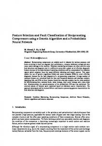
is true. Thus, the fault is detected for all logic value assignments to the X-sources. Then the next stuck-at fault is analyzed. If OPDD is empty and OPD is not empty, the stuck-at fault is marked as PD and the algorithm proceeds with the next stuck-at fault. If the current fault is neither marked DD nor PD and OPPD is not empty, the SAT solver is used to determine if one of the outputs in OPPD belongs to REXf (p). Note that this step is performed only if the fault is not yet marked as PD. If one output of OPPD is member of REXf (p), the fault is marked as PD. In the case that all outputs in OPPD belong to FEXf (p), the fault remains unmarked and undetected. V. E XPERIMENTAL R ESULTS The presented algorithm has been tested and applied to ISCAS benchmark and large industrial circuits from NXP. The experiments were run on an AMD Opteron CPU with 2.3 GHz. A. Reduction of Unknown Output Values The exact logic simulation algorithm of Section III efficiently computes the exact output values of the circuit for a test set. This is important for BIST and EDT environments to avoid unnecessary DFT overhead for X-masking or Xblocking structures, and overmasking of FEX-valued outputs. For the considered circuits, three simulation runs are performed and averaged. In each run, a fixed percentage of the controllable circuit inputs is randomly selected as X-sources (X-ratio). Then, a test set of 1 000 random patterns is analyzed. The difference in the number of PEX outputs of a 3-valued simulation and the REX outputs of the exact analysis is compared.

X-output reduction (%)

30 25 20 15 10 5 0

Fig. 4.

0

20

40 60 X-sources (%)

80

100

Reduction of unknown output values of ISCAS circuit c7552.

TABLE I R EDUCTION OF UNKNOWN VALUES AT THE OUTPUTS FOR 1 000 TEST PATTERNS AND 5% X- SOURCES . Circuits c6288 c7552 cs09234 cs13207 cs15850 cs35932 cs38417 cs38584 p35k p45k p77k p78k p81k p89k p100k p141k p267k p286k p295k Average

PEX 23 387 11 826 16 839 44 971 36 443 75 672 143 195 95 323 84 951 285 178 248 242 685 605 491 965 309 047 325 348 1 154 394 1 284 472 1 172 617 2 506 184 473456

Outputs REX Reduction (%) 15 215 34.9 9 387 20.6 15 608 7.3 39 854 11.4 34 999 4.0 75 672 0.0 122 760 14.3 91 877 3.6 80 240 5.5 215 963 24.3 195 593 21.2 454 267 33.7 384 691 21.8 255 373 17.4 277 661 14.7 919 633 20.3 1 124 916 12.4 758 732 35.3 2 102 686 16.1 377638 20.2

B. Exact Fault Simulation This section presents the increase of fault coverage of a test pattern set due to the non-pessimistic analysis with the

100 Exact algorithm Run time exact algorithm 80 Algorithm in [12]

14 12 10

60

8 6

40

4

20

2 0

Run time (s)

Similar experiments have been conducted for the other circuits as well. Due to limited space, we only present results for the case of 5% X-sources in Table I. Column ‘Circuit’ contains the circuit name. Column ‘PEX’ and ‘REX’ show the absolute number of unknown values at the outputs for the test set computed by 3-valued simulation respectively the exact algorithm. In a BIST architecture, only these REX outputs have to be masked for the computation of a signature. The last column in the table contains the reduction of X-values at the circuit outputs. In average, the number of X-values is reduced by 20.2%.

proposed algorithm. Similar to the previous section, three simulation runs are performed per circuit and averaged. In each run, a fixed percentage of the controllable circuit inputs is randomly selected as X-sources. Then, the fault coverage of a test set of 1 000 random patterns is computed using 3-valued fault simulation and the proposed exact algorithm. For circuit c7552, Figure 5 depicts the increase in fault coverage of the exact algorithm w. r. t. 3-valued fault simulation for different X-ratios, and the runtime in seconds. The circles indicate the increase of fault coverage if 1 000 test patterns are analyzed exactly. The exact algorithm increases fault coverage by up to 14.2%. The highest increase of fault coverage is achieved when approximately 10% of the inputs are X-sources. Compared with the approximate hybrid fault simulation of [12], the exact algorithm reveals that up to 30% additional faults are actually detectable with the test set. Additionally detected stuck-at faults (%)

Figure 4 shows the reduction of the number of unknown outputs for ISCAS circuit c7552 for different X-ratios. The diagram shows that the number of unknown values is reduced by more than 25% for the X-source scenarios with 1% and 7% X-sources. The reduction decreases to 0% if nearly all inputs are X-sources.

0

20

40 60 X-sources (%)

80

0 100

Fig. 5. Increase in stuck-at fault coverage by accurate fault simulation with 1 000 random test patterns for circuit c7552.

The runtime of the proposed algorithm reaches the maximum of 91s at an X-ratio of about 35%. Compared to the method of [12] with a runtime of 2 749s, the proposed algorithm is 30× faster. For small X-ratios, the runtime is low since RSS uncovers many FEXs at simple X-reconvergences. If the SAT solver is required, the size of the CNF formula is small. For high X-ratios, the pattern parallel simulation of random assignments to X-sources determines most of the REX signals. Table II reports the results for a larger set of ISCAS and industrial circuits. Due to limited space, the results are limited to the case of 5% X-sources. For each circuit, the table shows the absolute number of stuck-at faults. Column ‘3-val. Fsim.’ shows the absolute number of detected faults and the fault coverage in % of 3-valued fault simulation. The number of additionally detected faults and fault coverage increase by the exact algorithm according to equation (1) is given in column ‘∆ Exact sim. DD.’ Column ‘Exact sim. PD’ lists the number and ratio of faults marked as potential detect (PD) according to equation (2). The last column lists the runtime for the exact analysis in seconds. On average, 3-valued fault simulation computes the coverage of the test sets to 67.2%. The exact fault simulation proves that an additional 1.8% of the faults are detected by the test sets. The increase in additionally detected faults is very high

TABLE II D ETECTED STUCK - AT FAULTS BY A TEST PATTERN SET WITH 1 000 PATTERNS AND 5% X- SOURCES . Circuit c6288 c7552 cs09234 cs13207 cs15850 cs35932 cs38417 cs38584 p35k p45k p77k p78k p81k p089k p100k p141k p267k p286k p295k Sum

Number faults 8 704 9 756 13 892 20 246 24 571 52 225 56 761 54 153 110 494 107 814 186 645 225 476 272 322 228 570 247 376 434 363 640 221 949 733 728 246 4 371 568

3-val. Fsim. Num. F.C.(%) 4 296 49.4 5 546 56.8 85 67 61.7 14 766 72.9 19 668 80.0 41 391 79.3 46 279 81.5 44 459 82.1 47 212 42.7 63 754 59.1 85 995 46.1 189 431 84.0 133 617 49.1 130 985 57.3 173 237 70.0 328 111 75.5 456 456 71.3 685 249 72.2 458 122 62.9 2 937 141 67.2

∆ Exact sim. DD Num. F.C.(%) 3 977 45.7 856 8.8 91 0.7 193 1.0 245 1.0 0 0.0 275 0.5 100 0.2 1 973 1.8 1 221 1.1 1 661 0.9 18 681 8.3 3 116 1.1 2 473 1.1 8 694 3.5 10 402 2.4 7 184 1.1 13 116 1.4 4 125 0.6 78 383 1.8

for the multiplier c6288 due to high signal observability and propagation of many X-values in the pessimistic simulation. The results also show that a noteworthy amount of stuck-at faults of 5.7% on average can be classified as potential detect. The runtime of the algorithm for the considered ratio of Xsources ranges from 4 milliseconds up to 190 seconds for a single pattern. VI. C ONCLUSIONS The work presented the first stuck-at fault simulator, which is able to calculate the exact fault coverage of a test pattern set in the presence of unknown values. The simulator employs logic and restricted symbolic simulation to classify as many signal states as possible without invoking formal SAT reasoning. Incremental SAT solving is utilized only to exactly analyze the remaining signal states. The usage and runtime of the SAT-solver and the size of the CNF formulae are strongly reduced by considering the simulation results and employing incremental SAT techniques. The algorithm is able to handle large industrial circuits. ACKNOWLEDGMENT The authors thank Tobias Schubert for his SAT-solver Antom and related support. This work was partially supported by the German Research Foundation (DFG) under grants BE 1176/14-2 and WU 245/5-2. R EFERENCES [1] E. G. Ulrich and T. Baker, “The concurrent simulation of nearly identical digital networks,” in Papers on Twenty-five years of electronic design automation, ser. 25 years of DAC, 1988, pp. 318–323. [2] J. Waicukauski, E. Eichelberger, D. Forlenza, E. Lindbloom, and T. McCarthy, “Fault simulation for structured VLSI,” VLSI Systems Design, vol. 6, no. 12, pp. 20–32, 1985. [3] K. Antreich and M. Schulz, “Accelerated fault simulation and fault grading in combinational circuits,” IEEE Trans. CAD, vol. 6, no. 5, pp. 704 – 712, september 1987. [4] H. Lee and D. Ha, “An efficient, forward fault simulation algorithm based on the parallel pattern single fault propagation,” in Proc. International Test Conference (ITC), oct 1991, pp. 946–955.

Exact sim. PD Num. F.C.(%) 80 0.9 1 615 16.6 816 5.9 679 3.4 588 2.4 161 0.3 1 504 2.6 1 125 2.1 5 083 4.6 16 339 15.2 10 537 5.6 6 368 2.8 30 284 11.1 13 784 6.0 18 315 7.4 18 943 4.4 42 798 6.7 43 441 4.6 37 378 5.1 249 837 5.7

Run time (s) 4 4 8 12 10 62 80 54 604 975 26 338 3 461 100 510 3 591 17 411 59 375 85 520 190 158 149 942 638 120

[5] M. Naruse, I. Pomeranz, S. Reddy, and S. Kundu, “On-chip compression of output responses with unknown values using LFSR reseeding,” in Proc. of the IEEE International Test Conference, 2003, pp. 1060–1068. [6] S. Mitra and K. S. Kim, “X-compact: an efficient response compaction technique,” IEEE Trans. CAD, vol. 23, no. 3, pp. 421–432, 2004. [7] M. H. Schulz, E. Trischler, and T. M. Sarfert, “Socrates: a highly efficient automatic test pattern generation system,” IEEE Trans. on CAD of Integrated Circuits and Systems, vol. 7, no. 1, pp. 126–137, 1988. [8] S. Kajihara, K. K. Saluja, and S. M. Reddy, “Enhanced 3-valued logic/fault simulation for full scan circuits using implicit logic values,” in Proc. IEEE European Test Symposium (ETS), 2004, pp. 108–113. [9] S. Kang and S. A. Szygenda, “Accurate logic simulation by overcoming the unknown value propagation problem,” Simulation, vol. 79, no. 2, pp. 59–68, 2003. [10] J. Carter, B. Rosen, G. Smith, and V. Pitchumani, “Restricted symbolic evaluation is fast and useful,” in Proc. IEEE International Conference on Computer-Aided Design (ICCAD), nov 1989, pp. 38 –41. [11] R. E. Bryant, “Graph-based algorithms for boolean function manipulation,” IEEE Trans. on Computers, vol. 35, no. 8, pp. 677–691, 1986. [12] M. A. Kochte and H.-J. Wunderlich, “SAT-based fault coverage evaluation in the presence of unknown values,” in Proc. Design, Automation and Test in Europe (DATE’11), 2011, pp. 1–6. [13] A. Jain, V. Boppana, R. Mukherjee, J. Jain, M. Fujita, and M. Hsiao, “Testing, verification, and diagnosis in the presence of unknowns,” in Proc. VLSI Test Symposium, 2000, pp. 263–268. [14] C. Wilson, D. Dill, and R. Bryant, “Symbolic simulation with approximate values,” in Formal Methods in Computer-Aided Design, ser. LNCS, W. Hunt and S. Johnson, Eds. Springer Berlin / Heidelberg, 2000, vol. 1954, pp. 507–522. [15] C. Scholl and B. Becker, “Checking equivalence for partial implementations,” in Proc. Design Automation Conference (DAC), 2001, pp. 238– 243. [16] S. Kundu, I. Nair, L. Huisman, and V. Iyengar, “Symbolic implication in test generation,” in Proc. Conference on European Design Automation, 1991, pp. 492–496. [17] B. Becker, M. Keim, and R. Krieger, “Hybrid fault simulation for synchronous sequential circuits,” Journal of Electronic Testing: Theory and Applications (JETTA), vol. 15, no. 3, pp. 219–238, 1999. [18] M. A. Kochte, S. Kundu, K. Miyase, X. Wen, and H.-J. Wunderlich, “Efficient BDD-based fault simulation in presence of unknown values,” in Proc. IEEE 20th Asian Test Symposium (ATS11), 2011. [19] T. Schubert, M. Lewis, and B. Becker, “Antom—solver description,” SAT Race, 2010. [20] G. Tseitin, “On the complexity of derivation in propositional calculus,” Studies in constructive mathematics and mathematical logic, vol. 2, no. 115-125, pp. 10–13, 1968.