EXEMPLAR-BASED IMAGE INPAINTING: FAST PRIORITY AND ... - Inria

2012 IEEE INTERNATIONAL WORKSHOP ON MACHINE LEARNING FOR SIGNAL PROCESSING, SEPT. 23–26, 2012, SANTANDER, SPAIN

EXEMPLAR-BASED IMAGE INPAINTING: FAST PRIORITY AND COHERENT NEAREST NEIGHBOR SEARCH R. Mart´ınez-Noriega, A. Roumy

G. Blanchard

INRIA Campus Universitaire de Beaulieu 35042 Rennes-Cedex, France

Universitat Potsdam Institut f¨ur Mathematik Am neuen Palais 10, 14469 Potsdam, Germany

ABSTRACT Greedy exemplar-based algorithms for inpainting face two main problems, decision of filling-in order and selection of good exemplars from which the missing region is synthesized. We propose an algorithm that tackle these problems with improvements in the preservation of linear edges, and reduction of error propagation compared to well-known algorithms from the literature. Our improvement in the filling-in order is based on a combination of priority terms, previously defined by Criminisi, that better encourages the early synthesis of linear structures. The second contribution helps reducing the error propagation thanks to a better detection of outliers from the candidate patches carried. This is obtained with a new metric that incorporates the whole information of the candidate patches. Moreover, our proposal has significant lower computational load than most of the algorithms used for comparison in this paper. Index Terms— exemplar, inpainting, coherence, priority 1. INTRODUCTION The purpose of inpainting is to filling-in the missing part of an image. Diffusion-based inpainting preserves the structure (i.e. lines and object contours) by propagating the isophote (a line of equal luminance) in the unknown region (see the seminal work [1] and the overview in [2]). By construction, this approach achieves excellent results when the missing region is small. In this paper, we focus on filling-in larger regions1 . This problem occurs when blocks of data have been lost in transmission, or intentionally pruned for compression, or when an unwanted large object has to be removed. In this context, the missing part contains both image structure and texture. State-of-the-art methods are exemplar-based inpainting [3] and were inspired by texture synthesis algorithms [4, 5, 6]. Exemplar-based inpainting fills the holes in an image by searching similar information on the known region and simply copy it to the unknown region [3] as is done in texture synthesis [5, 6]. The previous premise is based on the fact that natural images contain redundant or very similar information [7]. Greedy inpainting using exemplars, also known as patches, consists of two major steps: select the patch to be filled, and propagate the texture and structure. The former step selects patches with mostly linear structures by giving them higher priority. The latter is related to the selection of the 1 This

problem is also known as image completion

c 978-1-4673-1026-0/12/$31.00 2012 IEEE

K-most similar patches from which the information is copied. These two steps are iterated until the holes in the image are fully restored. The contribution presented in this paper is twofold. We first propose an improvement to the priority order proposed by [3]. More precisely, [3] proposes a simple but efficient priority criterion based on the isophote strength and on the angle between the isophotes and the boundary (between the known and the unknown region). Different improvements have been proposed that can be classified with respect to their complexity. For instance, [8, Chapter 6] proposes to add a term that counts the number of known pixels which belongs to an edge. Therefore an edge detection algorithm has to be added. [9] proposes to solve the global inpainting optimization problem with a message passing. To make the solution sequential, a scheduling is proposed that requires the computation of many distances at the initialization. More precisely, for each patch located at the boundary between the known and the unknown region, the distance between this patch and all known patches have to be computed. In [10], only patches located in a neighborhood window are tested, in order to reduce the number of distances to compute. However, the priority term [10] still increases significantly the complexity of the priority term computation. In this paper, we show that by better combining the two priority terms proposed by [3], we get significantly improvements in the structure propagation without any complexity increase. Our second contribution concerns spatial coherence. Different attempts have been proposed to increase the spatial coherence of inpainted images. Some of them reduce the search of candidate patches i.e. the patches from which the information is copied (spatial neighborhood in [10] or parents of the spatial neighborhood [6]). Other methods, impose that candidates for overlapping patches are coherent either through an energy term [2] or through a graph that represents the spatial connection between the underlying patches of an image [9]. Interestingly, all these methods, when they select a candidate patch, base their choice on partial data of the patch. More precisely, only the pixels that correspond to the known pixels of the patch to be filled in, are used. Instead, we propose a novel criterion that takes into account all the pixels in the candidate patch. The idea is to include the probability density function (pdf) of the patches to the metric used for measuring the similarity. With this improvement we are able to better detect outliers from the candidate patches and therefore reduce the error propagation which commonly affects algorithms based on exemplars. The paper is organized as follows. In Sec. 2 the overall algorithm is introduced. Detail explanation of the two major steps: filling order

Ωn denote the known and unknows regions at iteration n, respectively. The goal is to infer f : {0, ..., 255}d×|Ψp ∩Ωn | −→ {0, ..., 255}d×|Ψp | x = P Ψp 7−→ y

(a) (b) (c) Fig. 1. Exemplar based inpainting. (a) Original image I with the unknown region Ω, its contour δΩ, and the known region Ω. (b) K patches Ψq i are found to synthesize the unknown area of the patch Ψp , with p ∈ δΩ. (c) Example of the imaginary edge that helps the pdf computation for patches classified as structures. and propagation of textures-structures are described in Sec. 3 and Sec. 4 respectively. Sec. 5 presents experimental results, and Sec. 6 concludes the paper. 2. DEFINITIONS AND OVERALL ALGORITHM Throughout the paper, the function I define an image (1). Let pixel denotes the pixel position of the image, whereas pixel value refers to as the value taken by the image at this pixel. More precisely, a pixel is mapped to a scalar (d = 1) for a gray level image and a vector (d = 3) for a color image: I : I −→ {0, ..., 255}d p 7−→ Ip

(1)

The image domain I contains missing regions, i.e. holes on the image whose information is unknown. Define the unknown region as Ω, and the known region as Ω. The two regions define a partition of the whole image domain and are separated by a so called contour δΩ (also known as the “fill front”), see Fig.1-(a). Our algorithm is patch based, as it was first introduced in [5] for texture synthesis. The patch Ψi is a square subregion of I centered at pixel i. In practice, the size of Ψi is decided to be slightly larger than the largest distinguishable texture element. In our case, and for the remaining of the paper, the size of the patches is 9 × 9 pixels. The algorithm aims to complete I by filling Ω with visually plausible information taken from Ω. This task is carried out by iterating two main steps: decision of the filling order and selection of suitable information to fill in the unknown part. More precisely, the algorithm first selects the patch Ψp , with p ∈ δΩ, whose filling priority is maximum among the patches of the fill front. Notice that Ψp contains a region already filled (known region) and a region where there is no information (unknown region). Then, the K-most similar patches Ψq i to Ψp are found, where i = 1, 2, . . . , K and Ψq ∈ Ω, Fig 1-(b). Finally, the Ψq i are linearly combined to predict the unknown region of Ψp . These steps are iterated until the unknown region Ω is filled. This two step approach (filling order and information propagation) has been originally proposed in [3]. By construction, the algorithm is sequential. At each iteration n, the missing part of the current processed patch is inferred. Formally, let P be the matrix that selects the known pixels from the current patch Ψp . Let Ωn and

(2)

In [3], the function f (2) is estimated with a 1-nearest neighbor (NN) approach. Further improvements have been proposed which are based on K-nearest neighbor (K-NN) search and Kernel smoothers [11, Chapter 6]. A Gaussian Kernel is used in [12], a Kernel with sparse constraint is used in [10], whereas the weights results from a constrained least square optimization in [8, Chapter 6]. We do not consider here the Kernel in [10], since it is well suited to the sparsity filling order proposed in the same paper. Instead, we consider Kernels that use Criminisi’s filling order and choose the one that give the best results that is [8]. We now explain in detail the two main steps of the algorithm: selection of filling order, and propagation of texture-structure. 3. FILLING ORDER Previous works, [3, 8, 9], have shown that filling order is crucial for exemplar-based algorithms. The most popular idea hitherto is to propagate linear structures first and then textures, in such a way that the formation of prominent peninsulas in the fill front are avoided. In this Section, we introduce our definition of filling order that better encourage the propagation of structures before the synthesis of textures. Given the patch Ψp for some p ∈ δΩ, Criminisi et al. [3] proposed a priority for the filling order P (p) based on the product of two terms P (p) = C(p)D(p). (3) The first term, C(p), is the confidence term and quantifies the belief we have in the known information contained in Ψp . The second term is the data term and it is a function of the strength of isophotes hitting the front δΩ at each iteration, and it is the responsible of encourage the propagation of linear structures. The terms are defined as follows: P |∇Ip⊥ · np | q∈Ψp ∩Ω C(q) C(p) = , D(p) = (4) |Ψp | α where |Ψp | is the area of Ψp , α is a normalization factor (e.g., α = 255 for a typical gray-level image), and np is a unit vector orthogonal to the front δΩ in the point p. The function C(·) is initialized with C(p) = 1, ∀p ∈ Ω and once a patch has been filled, say Ψp , the confidence term of the filled pixels is set to the belief associated to the patch: C(q) = C(p), ∀q ∈ Ψp ∩ Ω. Therefore, the first term C(p) counts the ratio between the belief we have on the current patch and the belief associated with a perfect known patch (a known pixel has belief 1). The second term is defined on [0, 1], and it increases with the norm of the gradient |∇Ip | (strong isophote) and also if this isophote becomes more perpendicular to the contour. Therefore, when D(p) → 1, the patch is very likely to have a strong linear structure. Although (3) tends to propagate linear structures, it often fails to fully reconstruct the edges of natural images. Then, we propose to amplify the data term in a nonlinear fashion by modifying (3) in the following way:   D(p) . (5) Pˆ (p) = C(p) exp 2σ 2

The rationale for this exponential amplification is that we seek for a filling-order that promote the early propagation of strong structures. However we would like to keep the concentric filling order when regions are smooth. The exponential in (5) reaches this compromise since it highly increases the influence of the data term when D(p) → 1 (strong linear structures), whereas no amplification is performed when D(p) → 0 (smooth region). Another rationale is that the confidence term C(p) (4) decreases exponentially with the distance between the current patch and the contour δΩ. Therefore, in order to compensate for the high values of C(p) near the contour, an exponential amplification of data term D(p) (4) has to performed. Finally, in order to be an amplification, the function  f ofthe data term has to satisfy f (D) ≥ D. The function exp D(p) satisfy 2σ 2 this constraint.2 4. PROPAGATING TEXTURE AND STRUCTURE Once the patch Ψp with maximum priority has been selected, the next step is to synthesize its missing region Ψp ∩Ω. This is achieved by searching K similar patches Ψq i , where Ψq i ∈ Ω and i = 1, 2, . . . , K, to the patch to be filled Ψp . Then, the unknown region of Ψp is filled with equivalent information extracted from the K similar patches Ψq i , e.g. using a linear combination or simply copy the information from the best match. 4.1. New metric for the selection of similar patches The most popular way to chose K-similar patches is to select those patches that minimize the sum of square distance (SSD) [3], formally Ψq i = arg min dSSD (P Ψp , P Ψq ),

(6)

Ψq ∈Ω

where dSSD is the SSD distance and the matrix P extracts the known region from the patch Ψp (pixels known or already filled). However as pointed out in [2], this criterion can select patches that are visually different and the final result is not visually coherent. Moreover, dSSD (P Ψp , P Ψq ) is a pixel-by-pixel metric constrained to the region defined by P and it does not use the whole information contained in Ψq . We propose to replace dSSD in (6) by a more robust metric (7) that uses a combination of SSD and the Hellinger distance in the following way: d(Ψp , Ψq ) = dSSD (P Ψp , P Ψq ) × dH (Ψp , Ψq ),

(7)

where dH stands for the Hellinger distance. The latter defines how similar the pdfs of two patches are. The motivation for such a metric is that with pdfs we can compare patches of different sizes and therefore include the whole information of the patch Ψq . Note that this is not the case with dSSD since the computation is performed on the known region defined by P Ψq . The values taken by dH are between [0, 1] and then, (7) can be seen as a weighted SSD. Hellinger distance is defined as: v u N u X p ρp (i)ρq (i), (8) dH (Ψp , Ψq ) = t1 − i=1 2 Note that other exponential functions exist, as D(p)n . But these functions do not satisfy the above mentioned amplification property.

where ρp , ρq are the pdf of the patches Ψp , Ψq respectively. Those pdfs are computed with the normalized histograms of the patches. In total, N bins are used to compute the histograms (e.g. for color images in RGB format, N/3 bins are used for each channel). The normalization is given according to the number of elements of each patch and the number of color dimensions. In [2], a similar metric to (7) was proposed. However, the originality of our proposal is based on how the term ρp · ρq from (8) is computed, and used to achieve two goals: reduction of error propagation and increase the accuracy of the prediction. Moreover, we introduce a distinction between texture and structure patches that dictates the way in which the pdfs are computed. For textures patches we are interested to include a coherence constraint in order to reduce the error propagation, whereas with structures patches the pdfs are computed in such a way to increase the accuracy of the prediction. Patch classification: texture vs. structure Let Ψp be the patch to be filled, and which has two well defined regions, the known part P Ψp and the unknown P Ψp . In order to decide if the patch is a texture or structure patch, we search for the three biggest gradient vectors inside P Ψp and average them. If the magnitude of the average gradient vector is higher than a threshold T the current patch Ψp is considered as structure patch, otherwise as texture one. We now define how to compute ρp · ρq depending on the nature of the patch, i.e. texture or structure. Hellinger distance for Structure patches We need to compare the pdfs of patches that are defined on different regions: known region for the current patch Ψp , whereas whole region for the candidate patches Ψq , taken from the dictionary. Therefore, in order to be comparable3 , we need to infer the pdf of the current patch Ψp on the whole region. To do so, we need to review what a structure patch is. A structure patch has gradient vectors with big magnitude that might indicate the presence of an edge, or in other words, two regions that contrast in colors. Our idea is to divide the current patch Ψp in two regions r1 and r2 , such that pixels in the same region have similar colors, see Fig. 1-(c). For simplicity and also because the patches are rather small (9 × 9 is a current patch size), we assume that the boundary between the two regions is linear. In order to construct this linear edge across Ψp , we first compute the average vector of the three biggest gradient vectors4 of P Ψp . Then, the edge is the line defined by the average vector and xc , the center of the three pixels with biggest gradient vector. The pdf of the current patch Ψp inferred on the whole domain can not be computed. Let R be the matrix that extracts the information contained in r1 and R for r2 . Then, the pdf of Ψp is computed as |RΨp | |RΨp | ρp = ρp 1 + ρp 2 , (9) |Ψp | |Ψp | where: ρp 1 =

H(P Ψp ∩ RΨp ) , |P Ψp ∩ RΨp |

ρp 2 =

H(P Ψp ∩ RΨp ) . |P Ψp ∩ RΨp |

As for the candidate patch Ψq , since the patch is known on the 3 Note that the usual way to make the patches comparable, is to restrict the computation to the known region. But this is exactly what we want to avoid. 4 For the sake of brevity, we refer to the gradient vector with biggest magnitude value as the biggest gradient vector.

5. EXPERIMENTS AND COMPARISONS

whole region, the pdf is the usual one. Formally, ρq =

H(Ψq ) . |Ψq |

(10)

Finally, the combined metric (7) contains the Hellinger distance between the histograms (9) and (10). Therefore, patches selected with (7) are more coherent with the current patch since it ensures that even on the unknown region, the candidate patch is similar to the current patch. The rationale to reinforce the coherence as shown above is to reduce the error propagation observed in many exemplarbased inpainting algorithms. Hellinger distance for Texture patches Texture patches are rather smooth and there is no need to separate the patch into two regions. The pdf computation for a texture patch is as follows. Therefore, computations of the histograms of P Ψp (on known region) and Ψq (on the whole region) might sufficient. However, since the known regions of Ψp and Ψq are already compared in the SSD, a way to enforce coherence is to favor patches Ψq whose region P Ψq (in the unknown area of Ψp ) is similar to P Ψp . Formally, given the patch Ψp , the pdf of Ψp is computed as: ρp =

H(P Ψp ) , |P Ψp |

(11)

where H is a function that computes the histogram, and | · | is the area of P Ψp . As for the candidate patch Ψq , where Ψq ∈ Ω, we define H(P Ψq ) ρq = . (12) |P Ψq | Finally, the combined metric (7) can be seen as a weighted SSD distance that is biased toward patches Ψq which are coherent. Here again, the goal is to avoid the error propagation phenomenon observed in many exemplar-based inpainting algorithms.

4.2. Synthesis Once the K nearest patches Ψq i are found either using the texture or structure definition, we use a linear combination of the patches to finally obtain the prediction of the missing pixels: P Ψp =

K X

ωi P Ψqi .

i=1

As in [8], the coefficients ω ~ are obtained by solving min k ω ~

K X

ωi P Ψqi − P Ψp k2

s.t.

i=1

K X

ωi = 1.

(13)

i=1

The optimization problem given in (13) can be solved in the same fashion as applied in local linear embedding (LLE) for data dimensionality reduction. In our case, the Gram matrix is G = (P Ψp 1 − X)T (P Ψp 1 − X), where X is a matrix with columns {P Ψq 1 , P Ψq 2 , · · · , P Ψq K } and 1 is a column vector of ones. Then it has a close form solution ω ~ =

G−1 1 1T G−1 1

.

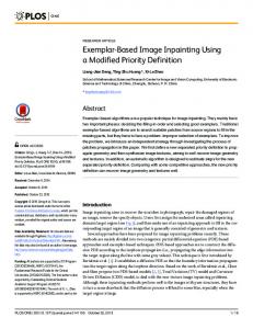
In this Section, we present simulation results of our algorithm on natural images, and comparisons with other popular algorithms from the literature. We also show empirical evidence of the advantages conveyed by the ideas proposed in this work i.e. improved filling order and spatial coherence. Fig. 2 is a summary of inpainted images using different methods considering that the light green region shown in (a) is the missing information. We compare our proposal with three other patch based inpainting algorithms. (b) is the seminal proposal of [3] in which the filling order is decided with (3) and the synthesis is achieved by copying the information from the most similar patch only. Turkan [8], (c), uses edge detection to augment the priority defined in [3] and the synthesis is produced by a linear combination of patches. Recently, Adobe Photoshop has introduced a tool called PatchMatch [13] to inpaint missing regions on images. The inpainted results of this tool is reported in (d). Finally, the last three columns are our results. (e) is the result of the algorithm as exactly described in this paper. In (f), we explore a different metric, structural similarity index (SSIM) [?] that is more consistent with human eye perception than SSD. Therefore, SSIM replaces SSD for the selection of the most similar patches. As for the weight computation in the synthesis step, SSIM cannot be used directly by LLE, since LLE directly refers to euclidean distances. Therefore in (f), the K-most similar patches were selected with SSIM and then, their SSD were used to compute the weights in the synthesis. In order to involve only the SSIM in the weight computation, we decide to change LLE by nonlocal means (NLM) [12]. This result is shown in column (g). The first row corresponds to a block erasure scenario5 . In this context, the ground truth is known, which allows to compute a PSNR value after reconstruction of the missing part. In all the other rows, an unwanted large object has to be removed and therefore no PSNR can be computed. The strongest characteristic of our algorithm is to stop the error propagation that highly affect patch-based algorithms. This is more evident in the block erasure scenario, shown in the first row of Fig. 2, in which our algorithm outperforms other proposals by at least 12 dB. In general our proposal provides a better completeness of linear edges and a more natural look of the missing region. For example in the Bungee jumping image where the man is complety erased, [3] and PatchMatch [13] fail to complete the roof of the shelter. Instead, our result not only completes the edge but also provides more visually pleasant images than [8]. Visual coherence is only achieved with our proposal for the Soldier image. In this case, the horizontal edge between the grass and the wall on the left part is not linearly propagated by our algorithm because there is a stronger edge on the right part (black plastic bag and grass) that is filled in first. The image Bench was the toughest for all the algorithms, but our proposal is the only one to complete more naturally the edges of the bench. In the Jaguar image, our result is the only one which fully completes the tree branch and eliminates the propagation of errors in the leftupper region of the branch. SSIM metric is promising since it estimates perceived errors, a characteristic that matters in inpainting. However, SSIM is applied 5 This problem occurs when blocks of data have been lost in transmission, or intentionally pruned for compression.

16.5 dB

16.3 dB

Bungee jumping 17.5 dB

30.3 dB

30.2 dB

30.9 dB

Soldier

Bench

Jaguar

(a) Missing part (b) Criminisi [3] (c) Turkan [8] (d) PatchMatch [13] (e) Ours SSD (f) Ours SSIM (g) Ours SSIM-NLM Fig. 2. Comparison of inpainted images obtained with our proposals, (e)-(g), and popular algorithms from literature. In columns, (a) Light green color represents the missing region. (b) Algorithm proposed in [3]. (c) Inpainted images obtained with [8]. (d) Resulting images after inpainting with PatchMatch tool [13] from Adobe Photoshop. only on luminance value and therefore faces problems of color mismatch. This can be notice in (g) of Fig. 2-Soldier, where SSIM chooses patches with similar structure but different color for the wall. The same problem is shown in Soldier-(f) but reduced, because, in this case, SSIM is combined with SSD. We introduced two novel ideas to improve the performance of exemplar-based inpainting. First, a modified priority for the filling order has been introduced in order to better reproduce the edges in the missing part. Second, a novel way to select the candidate patches has been proposed in order to reduce the propagation of errors in the inpainted image. We now focus on the former one. Fig. 3 shows the filling order used by [3] and our algorithm. We represent the filling

order with a gray scale of colors. The darker patches correspond to places that are filled-in first. Unlike [3], our proposal better encourages the early propagation of linear structures without disturbing the concentric filling order in regions that are smooth. This trade-off between synthesis of structure-textures is important to obtain good performance. Since our proposal of filling order is based on increasing the influence of the data term D(p), one might think that the filling order which first propagates structures only, would produce better results. However allowing the structures or edges to fully drive the inpainting process is not efficient, because it causes the formation of peninsulas in the fill front, as observed in [3]. Our second contribution aims to reduce the error propagation

ity load is lower. Moreover, the improvement in the filling-in order does not increment the complexity. In this proposal, we used crossvalidation to compute the threshold T which distinguishes texture from structure patches, and the variance σ 2 that controls the amplification of the data term. An open problem is an easy way to tune the parameters or even avoid them. Further work includes improving the classification of the patches and the inpainting adapted to each class, in order to obtain a less parametric technique.

(a) Criminisi [3] (b) Our proposal Fig. 3. Filling order for the “Bungee jumping”. Darker patches are regions that are inpainted first. (a) Location of the patch

7. ACKNOWLEDGMENTS This work was supported by the ANR-09-VERS-019-02 grant (ARSSO project). The authors would also like to thank the reviewers for their comments that help improve the manuscript. 8. REFERENCES

(b) Patch to be filled.

[1] M. Bertalmio, G. Sapiro, V. Caselles, and C. Ballester, “Image inpainting,” in SIGGRAPH, 2000. [2] A. Bugeau, M. Bertalmio, V. Caselles, and G. Sapiro, “A comprehensive framework for image inpainting,” IEEE Trans. Image Process., vol. 19, no. 10, pp. 2634 –2645, Oct. 2010.

(c) dSSD

(d) Our metric

[3] A. Criminisi, P. Perez, and K. Toyama, “Region filling and object removal by exemplar-based image inpainting,” IEEE Trans. Image Process., vol. 13, no. 9, pp. 1200 –1212, Sept. 2004. [4] A. A. Efros and T. K. Leung, “Texture synthesis by non-parametric sampling,” in International Conference on Computer Vision, Sept. 1999. [5] Y. Xu, G. Guo, and H.-Y. Shum, “Chaos mosaic: Fast and memory efficient texture synthesis,” Tech. Rep., Microsoft Research, April 2000.

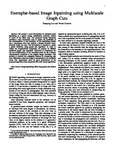
1 2 3 4 5 Fig. 4. Our metric produces better selection of candidate patches than dSSD . (a) The red square show the location to be filled. (b) Light green color is the region to be filled. (c) From left-to-right the five most similar patches to (b) chosen with dSSD . (d) Five most similar patches chosen with our metric. generated by the presence of outliers in the candidate patches when dSSD is used to select those patches. We propose a more robust metric (7) that account the whole information from the candidate patches. In Fig. 4 we show how our metric can better distinguish the outliers patches over the popular dSSD . We notice that patches chosen with dSSD contain artifacts that are not well suited for the neighborhood whereas our metric selects more visually pleasant patches.

6. CONCLUSION We proposed an inpainting algorithm that produces better completeness of linear edges and reduces the error propagation problem. The empirical results on natural images show better performance than well-known greedy algorithms, and better or similar performance than highly complex algorithms that need to inpaint the full missing part several times until convergence. Instead, our algorithm only needs to inpaint the missing region once and therefore the complex-

[6] M Ashikhmin, “Synthesizing natural textures,” in ACM Symposium on Interactive 3D Graphics, 2001. [7] M. Zontak and M. Irani, “Internal statistics of a single natural image,” in IEEE Conference on Computer Vision and Pattern Recognition (CVPR), June 2011. [8] M. Turkan, Novel texture synthesis methods and their application to image prediction and image inpainting, Ph.D. thesis, Univ. Rennes 1, Dec. 2011. [9] N. Komodakis and G. Tziritas, “Image completion using global optimization,” in IEEE Conference on Computer Vision and Pattern Recognition (CVPR), 2006. [10] Z. Xu and J. Sun, “Image inpainting by patch propagation using patch sparsity,” IEEE Trans. Image Process., vol. 19, no. 5, pp. 1153–1165, May 2010. [11] T. Hastie, R. Tibshirani, and J. Friedman, The Elements of Statistical Learning (2nd edition), Springer-Verlag, 2nd edition, 2008. [12] A. Wong and J. J. Orchard, “A nonlocal-means approach to examplar based inpainting,” in IEEE Int. Conf. Image Processing, 2008. [13] C. Barnes, E. Shechtman, A. Finkelstein, and D. B. Goldman, “Patchmatch: A randomized correspondence algorithm for structural image editing,” ACM Trans. Graph., vol. 28, no. 3, pp. 24:1–24:11, 2009.