ExOpaque: A Framework to Explain Opaque Machine Learning ...

ExOpaque: A Framework to Explain Opaque Machine Learning Models Using Inductive Logic Programming Yunsong Guo and Bart Selman Department of Computer Science Cornell University Ithaca, NY 14853, USA

Abstract

such as AdaBoost[11] and Bagging[2]. Among the more traditional machine learning models, decision tree is a nice example of an “understandable” model, as a human expert can easily interpret a decision tree’s classification behaviors by looking at the split nodes. People have worked at extracting a tree structured model from trained ANN [7] or SVM [9] with varying degrees of success. Methods that try to learn a simpler model to mimic the behavior of a complex meta-level model have also been proposed [4, 8]. We will discuss more of these models in the related work section. However, we feel that a framework which is applicable to general machine learning models and capable of explaining the behavior of a trained model for human understandability with careful evaluations is more than needed. Fortunately, understandability is the strength of rulebased learning applications, such as in [21, 12]. Inductive Logic Programming (ILP) [15], as one rule-based learning model, has shown its efficiency in inducing new hypothesis in various applications, especially in the field of molecular biology [19, 20]. In this paper, we will develop a framework that explains the behavior of a “black box” machine learning model using Horn clauses induced by an ILP system for interpretability. We also developed a method to decrease ILP’s dependence on background knowledge to produce accurate predictions on datasets where pre-defined background knowledge is hard to obtain. We will present evidences that by using our method the ILP system’s accuracy would converge to that of other highly accurate opaque machine learning models such as ANN and SVM. The paper is organized as follows: in the next section we will briefly present the ILP preliminaries; then we will illustrate what ExOpaque can learn from opaque models using a synthetic example in section 3; in section 4 we will describe the ExOpaque algorithm in details and conduct the experiment analysis in section 5; section 6 contains the method we propose to improve ILP accuracy without background knowledge using some of the ideas introduced in ExOpaque; section 7 talks about other related work in

In this paper we developed an Inductive Logic Programming (ILP) based framework ExOpaque that is able to extract a set of Horn clauses from an arbitrary opaque machine learning model, to describe the behavior of the opaque model with high fidelity while maintaining the simplicity of the Horn clauses for human interpretations. In addition, traditional ILP systems often utilize a set of background knowledge to make accurate predictions. We also proposed a new method to use generated artificial training examples and high-accuracy opaque models to boost the prediction accuracy of an ILP system when background knowledge is absent and hard to obtain.

1. Introduction As the field of machine learning prevails, tens of new models are being proposed each year with increasing complexity and improved performances. However, before we can automate some critical decision processes previously determined by human experts using a machine learning model, the experts need to understand what the model is doing even if the model has shown promising performances in objective tests such as cross validation. For example, in order to diagnose cancer for patients, the doctor can never completely rely on any machine learning model; rather, he may prefer to be provided with an “explanation” of a high accuracy machine learning model on the diagnosis task to aid his decision makings. Unfortunately, most of the machine learning models being proposed are not “transparent”, i.e, they are very hard for a human expert to understand by looking at the trained model: Artificial Neural Net (ANN) consists of a layered network configuration and a soft-margin Support Vector Machine (SVM) consists of quadratic optimization formulations with weight and slack variables[6], let alone other meta-level models 1

3. Synthetic Dataset Illustration

more details, and the paper is concluded with future issues pointed out in section 8.

In order to demonstrate the main idea and feasibility of using ILP to extract a set of Horn clauses that closely describes the behavior of an opaque machine learning model for human interpretation, we will use a toy example of learning the concept of “2-disks”. In this example, we are trying to learn whether it is stable to put one disk on the other, given the sizes of the 2 disks. It is stable only when the size of the first (lower) disk is no smaller than the second. Suppose each disk can take size 1, 2 or 3. We generated 50 random instances of this task, and used SVM to learn the concept. SVM gives 94% accuracy in 10-fold cross validation. Then we apply ExOpaque to learn from the instances together with SVM’s predictions. And the 6 learned Horn rules are as follows, which are the underlining concept of stability for 2-disk:

2. Inductive Logic Programming Preliminaries Inductive Logic Programming (ILP) is the study that combines inductive machine learning and logic programming. The general problem an ILP system is trying to solve can be described as follows: Given a set of examples E consisting of positive example set E + and negative example set E − , and background knowledge B, such that 1. ∀ e ∈ E − B 6` e, 2. ∃ e ∈ E + B 6` e;

1. 2. 3. 4. 5. 6.

To learn a hypothesis H satisfying 1. ∀ e ∈ E − B ∧ H 6` e, 2. ∀ e ∈ E + B ∧ H ` e. In other words, ILP’s task is to find new hypothesis H, which together with the background knowledge B entails all the positive examples but not any negative example. In the process of inducing new rules to include in the current hypothesis, 4 of Duce’s inductive inference rules presented below are often considered, where lower case letters represent single propositional variable and capital letters represent conjunctions of such variables. Absorption Identification Intra-construction Inter-construction

stable :- disk1(3) unstable :- disk1(1), disk2(3) unstable :- disk1(1), disk2(2) stable :- disk1(2), disk2(2) unstable :- disk1(2), disk2(3) stable :- disk2(1)

This toy example shows the idea of how we may use ExOpaque to explain an opaque model (SVM) given its behaviors (predictions) on original input instances. We rely on the fact that the opaque model is relatively accurate, otherwise what we can learn by ExOpaque is still reasonably close to the model but can be far away from the true concept.

4. ExOpaque Algorithm

p ← A, B q ← A p ← q, B q ← A

ExOpaque is presented in Algorithm 1. The different ways we construct training examples in step (∗ ) for an ILP system in ExOpaque will be described and validated in the experiment section. The ILP system we used in ExOpaque is Progol version 4.4 [13]. We use Progol to only find Horn clauses where the body elements are conjunctions of attribute values, and the head element is the class label. The Horn clause format is similar as in the synthetic example, which makes the learned set of rules easy to understand. When using ExOpaque returned rules to classify examples, the example’s attribute values are matched sequentially from the first rule, and the first matching Horn clause’s head part specifies the class label of the example. We also supply Progol all attribute values of constructed training examples as mentioned above with their class labels. The algorithm starts with the constructed supervised example set E, and applies ILP model to learn a set of Horn clauses to describe the set E. However, the set of Horn clauses is not guaranteed to classify all examples in E, since we do not include any default rule such as class(A, 1) :- , which in general does not offer more understanding on the

p ← A, B p ← A, q q ← B p ← A, q

p ← A, B p ← A, C q ← B p ← A, q q ← C

p ← A, B q ← A, C p ← r, B r ← A q ← r, C

In practical ILP systems such as Progol [13] and Golem [14], new clauses in the hypothesis are generated from the search in the lattice defined by the θ-subsumption relationship on the clauses, where the bottom of the lattice is the most specific clause generated from a ground example. And the search process is often exhaustive in the lattice, assessed by a heuristic measure (Progol) or a deterministic relative least general generalization (RLGG) of the bottom of the lattice (Golem). Due to space constraints, interested readers are encouraged to refer to [1] for more details of ILP theories and techniques. 2

behavior of the opaque model. Instead, we iteratively update E to be the examples left unclassified in the while loop. And k is the ratio of newly correctly classified examples to the increase of the size of the rule set. We stop the process and return the set of Horn clauses sequentially added in each iteration when either there is no more example to apply ILP to (E=∅) or the gain of classifying more examples correctly is not worth the increase in rule size compared to the previous iteration (c×k < k0 ), where c is a constant representing our willingness to trade-off rule size with fidelity in general.

Table 1. Dataset Size Train size Test size

Wine 120 58

Lung 22 10

Car 150 50

Balance 200 100

ExOpaque. In this section, when referred to, the size of training/testing set of each dataset is given in Table 1 We compare our results with decision tree J4.8 in WEKA, which is a java implementation of the C4.5 decision tree algorithm, in turns in both fidelity and learned rule size. Fidelity is a measure of how similar a learned model is to the original one. Since ExOpaque is trying to explain an arbitrary opaque model, fidelity is a very important measure of ExOpaque’s performance. Formally, given a set of examples x=(x1 ,. . . ,xT ), if the predictions of model M1 and M2 on x are y1 =(y11 ,. . . ,yT1 ) and y2 =(y12 ,. . . ,yT2 ), theP fidelity between M1 and M2 on dataset x is defined as T 1 i i i=1 ∆(y1 , y2 ) where ∆ is the normal 0-1 loss function. T As a decision tree size is not directly comparable to a set of Horn clauses, we translate each decision tree leaf node into a single Horn clause (body elements represent tree splits, and head element is the classification at leaf node), and the size of a decision tree is the sum of all such Horn clauses. The size of a Horn clause is defined as the number of body elements plus one, for example, A :- B, C is a Horn clause of size 3. In addition, although both ExOpaque and J4.8 provide explanations for opaque models, there are a couple of differences to note. Firstly, the rules provided by J4.8 are of equal importance, as no rule can be a generalization of another. While ExOpaque rules are ordered, as the later rules can be generalizations of earlier rules, which provides another level of freedom of manipulating the final rule set: since the earlier rules are more important (examples that can be classified by them would not be matched against later rules), we could prune part of the rules at the end without significantly damaging fidelity. Secondly, although in theory, given an example set with no contradictions (i.e, examples with identical attribute values but different class labels), a decision tree with exponential size can always achieve 100% fidelity, the tradeoff between tree size and fidelity in ExOpaque is explicitly controlled by the parameter c.

Algorithm 1 ExOpaque Framework Input:fully trained opaque model M , M ’s training set (optional), test set (optional) Output: a set of Horn clauses to explain the behavior of M for interpretability Construct the set of training examples T without class labels, according to the availability of M’s train/test set.∗ y ← M (T) E ← (T , y) k0 ← 0, k ← 0, R ← ∅ while E 6= ∅ and c × k ≥ k0 do k0 ← k S R ← R Horn clauses learned by ILP on E, let S be the size of the newly learned clauses E+ , E− ← examples in E that are correctly and incorrectly classified by R in terms of label y. |E

Iris 100 50

|

k ← S+ E ← E\E+ \E− end while Return R

5. Experiment Design and Results For the task of explaining a fully trained machine learning model, depending on the availability of the training and testing examples, we need to be able to handle 4 different situations: only the training examples are available, only test examples are available, both are unavailable and both are available. Throughout this section, in order to obtain representative results, we will use 5 different opaque machine learning models, including Artificial Neural Networks (ANN), Soft-Margin Support Vector Machine (SVM), AdaBoost with Decision Stumps (AdaStump), Bagging with Random Forest [3] (BagRF) and Naive Bayes (NB). We used the implementations of all the above models from WEKA [22], with WEKA default parameters. As ExOpaque is a general framework, we can choose to apply it to arbitrary models for human interpretability. The datasets are all from UCI machine learning repository [16], including Iris, Wine, Lung Cancer, Car and Balance datasets, which have a good mix of both discrete and continuous attribute values. [5] provides a recent comparison of supervised learning algorithms on various UCI datasets. Since most rule-based learning models require the attributes to be discrete, we discretize all continuous attributes using the standard Minimum Description Length Principle (MDLP) on supervised data [10] before applying

5.1. Only Training Set Is Available When we are trying to understand the behavior of a model handed to us with only the examples that the model was trained on, ExOpaque uses the training set with the predicted class labels by the opaque model. In other words, if (x,y) is the training set with y being the true class labels and 3

y being the predicted labels, we apply ExOpaque on (x,y) to obtain the set of Horn clauses H. The fidelity in percentage and rule size comparisons of H with J4.8 is presented in Table 2. Each entry in the table consists a pair of numbers, such as (100;99). The first number in the pair is the statistic of ExOpaque and the second number is of J4.8. From the table we see that ExOpaque is always able to provide high fidelity (above 96%) interpretations of the opaque models, while J4.8 has higher efficiency in providing more compact interpretations with lower fidelity.

ated independently, and each attribute value is selected uniformly at random among all feasible discrete values. And the size of random example set is equal to the original training set. ExOpaque is used to explain the random examples with predictions from various machine learning models. Results are presented in Table 4. In cases where both train set and test set are available, we can either choose to study the behavior of models on the training or test sets as described in the previous sections.

6. ILP Accuracy Improvement without Background Knowledge

5.2. Only Test Set Is Available When we only have the fully trained model and test examples, due to the fact that the test set size is often much smaller than that of the training set, we may not be able to learn a good explanation of the trained model’s behaviors from only the predictions on the test set. As a result, we need to first obtain additional examples of similar distributions as the test set. MUNGE [4] is a nice fit for this task, as it takes into a small set of examples and multiply the size of example set by generating additional examples based on the original ones. The outline of MUNGE algorithm for dataset with discrete attribute values is presented in Algorithm 2. We set

The background knowledge to an ILP system is often provided in logic programs, describing what we know as truth a priori before we see any example. Fort instance, in the task of grammar parsing, a piece of background knowledge can be given as N P (S1 , S2 ) :det(S1 , S3 ), noun(S3 , S3 ). The dependance on supplied background knowledge of an ILP system makes it less desirable in situations where such knowledge is hard to obtain. For example, in most of the UCI datasets, only the attribute values are available but not any pre-defined background knowledge. As a result, ILP is not often used for general prediction purposes on such datasets. However, as ILP possesses the understandability property, developing a systematic way to get around the problem of lack of background knowledge can be very useful. During our development of ExOpaque, we have devised a method to address this problem by making use of high accuracy opaque machine learning models to boost the prediction accuracy of an ILP system without using background knowledge. The idea is to generate additional training cases, and use the opaque models trained on original training examples to predict them. Then we take those predictions as class labels for the additional examples, and train ILP using these new examples together with the original training set. To our knowledge, we are the first to propose combining the predictions of high accuracy models with artificial instances to get rid of the background knowledge dependency by most ILP systems to make accurate predictions on test data. More generally, in situations where a model has some certain desirable properties (as understandability for ILP), but suffers from low prediction accuracy, we propose to use a high-accuracy model to construct random instances to improve the accuracy while maintaining the desired properties. We will show that by using additional artificial instances we indeed can increase the accuracy of an ILP system. In addition, experiment results also suggest that the accuracy of ILP converges to the accuracy of the opaque model given enough additional instances. The ILP model we used here is the same as in ExOpaque described in section 3, and we

Algorithm 2 MUNGE on discrete data Input:set of training examples T, size multiplier k, probability parameter p Output: Unlabeled training set of size k × |T | D←∅ for (i=1; i≤k; i++) do T0 ← T for all examples e in T 0 do e0 ← closest example of e in T 0 for all non-class attribute a of example e do with probability p, swap the value of attribute a of e and e0 end for end for S D ← D T0 end for Return D

p to be 0.3, and the multiplier parameter k of MUNGE to be the smallest integer that the resulted example set size is at least the size of original training set, assuming we know the size of the train set. We use Euclidean distances as the distances among examples in MUNGE. Then we apply ExOpaque on the newly generated example set with predictions by opaque models. The results are presented in Table 3, which are similar to when only training set is available as ExOpaque has high fidelity (100%) in every case, and the rule size difference between J4.8 and ExOpaque is not as large.

5.3. Both Training And Test Sets Are Unavailable When both training and test sets are missing, we have to generate random instances. Each random instance is gener4

Table 2. Train Set Available Only (ExOpaque; J4.8) F IDELITY I RIS W INE L UNG C AR BAL

ANN 100; 99 100; 99.17 100; 90.91 100; 95 98.5; 90

RULE S IZE I RIS W INE L UNG C AR BAL

SVM 100; 100 100; 100 100; 90.91 100; 93.33 100; 94

ANN 12; 8 25; 22 27; 12 92; 71 227; 83

SVM 6; 8 32; 22 27; 12 78;30 78; 63

A DA S TUMP 100; 100 100; 99.17 100; 100 100; 100 100; 100

BAG RF 100; 99 100; 99.17 100; 90.91 100; 94 96.5; 89.5

A DA S TUMP 6; 8 25; 17 17; 8 1; 1 10; 4

BAG RF 12; 8 25; 22 27; 12 96; 66 231; 66

NB 100; 99 100; 100 100; 90.91 100; 98 100; 97

NB 12; 8 31; 22 28; 8 65; 33 196; 91

Table 3. Test Set Available Only (ExOpaque; J4.8) F IDELITY I RIS W INE L UNG C AR BAL

ANN 100; 100 100; 99.43 100; 93.33 100; 97.33 100; 99

RULE S IZE I RIS W INE L UNG C AR BAL

SVM 100; 100 100; 98.28 100; 93.33 100; 99.33 100; 97

ANN 12; 19 26; 28 23; 13 80; 53 164; 178

A DA S TUMP 100; 100 100; 100 100; 100 100; 100 100; 100

BAG RF 100; 100 100; 99.43 100; 93.33 100; 98.67 100; 98.5

A DA S TUMP 6; 8 21; 17 24; 17 1; 1 10; 4

BAG RF 12; 19 20; 28 36; 24 67; 66 130; 86

SVM 6; 8 26; 28 24; 13 49; 47 115; 64

NB 100; 100 100; 99.43 100; 93.33 100; 98 100; 99 NB 12; 19 24; 33 25; 13 51; 54 127; 118

Table 4. Both Train And Test Set Unavailable (ExOpaque; J4.8) F IDELITY I RIS W INE L UNG C AR BAL

ANN 100; 92 100; 91.67 100; 100 100; 96 99; 94.5

RULE S IZE I RIS W INE L UNG C AR BAL

SVM 100; 93 100; 91.67 100; 100 100; 96 100; 96.5

ANN 82; 49 99; 97 19; 13 113; 64 195; 103

A DA S TUMP 100; 100 100; 99.17 100; 95.45 100; 100 100; 100

SVM 56; 23 75; 51 21; 13 52; 25 168; 65

A DA S TUMP 20; 19 61; 48 19; 13 1; 1 10; 4

5

BAG RF 100; 100 100; 95.83 100; 90.91 100; 94 98.5; 94 BAG RF 24; 19 71; 75 19; 8 82; 34 182; 83

NB 100; 98 100; 93.33 100; 100 100; 98 100; 97 NB 81; 73 37; 1 16; 8 61; 52 128; 81

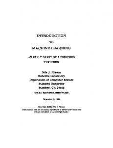
hensibility property. On the other hand, Munge-generated instances are not as good as random ones in this task as the performance converges to some lower accuracy very fast. This is due to Munge’s characteristic that it generates new instances based on the original training set, which limits its ability to provide instances scattered in a larger feasible attribute space. As a result, when the multiplier parameter k is large (greater than 3 in our experiments), the new instances are repetitive and condensed which will not provide additional information for ILP even if we further increase the additional training set size. It is surely interesting to take a close look at the other 2 plots (Car+ANN, Car+SVM). In the first one, we can still boost ILP’s accuracy by random additional instances, but the converged accuracy is still lower than that of the high-accuracy model (88.87% and 91.21%), while the Munge data is behaving strangely. We believe this is partially due to the fact that the base ILP accuracy is considerably high already, thus the margin for improvement is much smaller if compared with the Balance dataset. So within the small margin random fluctuations would appear to be more significant than before. While for the Car+SVM plot, since ILP base line is clearly higher than SVM base line, it is as expected that learning from a worse model would deteriorate accuracy. Again, Munge instances seem to be worse than random instances for the current task. In summary, from our experimental results, we propose to use additional random instances with predictions from models with significantly higher accuracy than ILP system, to train the ILP system in order to achieve comparable accuracy as the other model when background knowledge is not available.

Table 5. Model Performance Using Original Training Set Train Size 400 1000

Bal. Car

Test Size 225 728

ILP 52.00 87.07

Balance Dataset+ANN 95

90

90 ILP+Random ILP+Munge ILP Baseline ANN Baseline

Accuracy

80

85

75

70

70

65

65

60

60

55

ILP+Random ILP+Munge ILP Baseline SVM Baseline

80

75

50

55

0

500

1000

1500

2000

2500

3000

3500

4000

50

0

500

Car Dataset+ANN

1000

1500

2000

2500

3000

3500

4000

Car Dataset+SVM

92

88

91

ILP+Random ILP+Munge ILP Baseline ANN Baseline

90

Accuracy

SVM 90.22 84.34

Balance Dataset+SVM

95

85

ANN 92.89 91.21

86

84

ILP+Random ILP+Munge ILP Baseline SVM Baseline

89 88

82

87 80 86 78 85 84

0

500

1000

1500

2000

2500

3000

Additional Train Set Size

3500

4000

76

0

500

1000

1500

2000

2500

3000

3500

4000

Additional Train Set Size

Figure 1. Using Additional Training Set to Improve ILP Accuracy w/o Background Knowledge also use a training and a testing set to evaluate the prediction accuracy. We will use ANN and SVM as 2 representative relatively high accuracy opaque models and try to improve ILP accuracy on the Balance and Car datasets from UCI repository. We start with the full Balance and Car data sets and use ANN, SVM and ILP for the prediction task. The accuracies in percentage of the 3 models are presented in Table 5. We notice that ILP performance in prediction tasks without background knowledge is unstable, as it gives only 52% accuracy on Balance dataset but higher accuracy than SVM on Car dataset. For both datasets, we use random and MUNGE algorithm to generate additional instances. The results of ILP accuracy with these additional training examples can be found in Figure 1.

7. Related Work Trepan [7] is a model used to extract a decision-tree like structure from a trained neural network. While Trepan is also a model aimed at interpretability, its generalization power depends on a special m-of-n node which is a tree node that says “if at least m of the following n conditions are satisfied, take the left otherwise right branch”. Although this kind of explanation is normal in diagnostic decision criteria according to the authors, we feel such “m-of-n” conditions can be also confusing to people who are looking for more deterministic explanation of a model. In addition, it is not always possible to express one “m-of-n” condition as a simple Horn clause of polynomial size in n, so the total size of the structure extracted by Trepan is indeed more than the tree nodes have shown. Nevertheless, from the experiment results in [7], decision tree model size is better than Trepan model in half of the size comparisons. As a result, we based our comparison with J4.8. Trepan also makes use of artificially generated instances to compensate the decrease of training data to select split-

In the first 2 plots (Bal.+ANN and Bal.+SVM), we see that by introducing additional random instances with high accuracy model’s predictions, ILP’s performance actually converges to the high-accuracy model (from 52% to 92.44% for Bal.+ANN and to 90.22% for Bal.+SVM), without the need of background knowledge while maintaining the compre6

ting tests with the depth of the constructed tree structure. Bucilia et al [4] used a small size neural network to mimic the behavior of a complex ensemble model. They generated artificial data by random, Munge and NBE (Naive Bayes Estimation) methods. The artificial data is labeled by the ensemble model and used to train a neural network model. Experiment results show that the obtained neural network has similar performance as the ensemble model when Munge is used to generate the additional instances. While they also utilize the idea of using artificial data and predictions of a complex model to train another model, their goal is a smaller model rather than human comprehensibility in this paper. CMM (Combined Multiple Models) [8] uses C4.5Rules [17] to learn from a bagged ensemble of the same C4.5Rules base models, which are trained by bootstrap re-sampling of the original training set. In learning from the bagged ensemble CMM apply C4.5Rules on the original training set as well as instances constructed randomly with predictions of the bagged model. Experiments showed that the resulted model can retain 60% of the accuracy gain by bagged model relative to a single run of C4.5Rules. While CMM also returns a comprehensible model, it is not used to explain the behavior of the bagged model, or any other general opaque model; rather, it uses the information from a complex model to extract a simpler one and tries to maintain the accuracy benefit at the same time.

plex test conditions in the Horn clause body part, and make use of probabilistic ILP [18] to allow more freedom in the interpretation of ExOpaque returned explanations.

References [1] F. Bergadano and D. Gunetti. Inductive Logic Programming: From Machine Learning to Software Engineering. MIT Press, Cambridge, MA, USA, 1995. [2] L. Breiman. Bagging predictors. Journal of Machine Learning, 24(2):123–140, 1996. [3] L. Breiman. Random forests. Journal of Machine Learning, 45(1):5–32, 2001. [4] C. Bucilu, R. Caruana, and A. Niculescu-Mizil. Model compression. In Proceedings of the 12th ACM SIGKDD international conference on Knowledge discovery and data mining, pages 535–541, 2006. [5] R. Caruana and A. Niculescu-Mizil. An empirical comparison of supervised learning algorithms. In Proceedings of the 23rd international conference on Machine learning, pages 161–168, 2006. [6] K. Crammer and Y. Singer. On the algorithmic implementation of multiclass kernel-based vector machines. Joural of Machine Learning Research, 2:265–292, 2001. [7] M. W. Craven and J. W. Shavlik. Extracting tree-structured representations of trained networks. In Advances in Neural Information Processing Systems, pages 24–30, 1996. [8] P. Domingos. Knowledge acquisition from examples via multiple models. In Proc. 14th International Conference on Machine Learning, pages 98–106, 1997. [9] E. Douglas, D. Torres, M. Claudio, and S. Rocco. Extracting trees from trained svm models using a trepan based approach. In Proceedings of the Fifth International Conference on Hybrid Intelligent Systems, pages 353–360, 2005. [10] U. M. Fayyad and K. B. Irani. Multi-interval discretization of continuous-valued attributes for classification learning. In Proceedings of International Joint Conferences on Artificial Intelligence, pages 1022–1029, 1993. [11] Y. Freund and R. E. Schapire. Experiments with a new boosting algorithm. In International Conference on Machine Learning, pages 148–156, 1996. [12] N. Indurkhya and S. M. Weiss. Solving regression problems with rule-based ensemble classifiers. In Proceedings of the seventh ACM SIGKDD international conference on Knowledge discovery and data mining, pages 287–292, 2001. [13] S. Muggleton. Inverse entailment and Progol. New Generation Computing, Special issue on Inductive Logic Programming, 13(3-4):245–286, 1995. [14] S. Muggleton and C. Feng. Efficient induction of logic programs. In Proceedings of the First Conference on Algorithmic Learning Theory, pages 368–381, Tokyo, 1990. [15] S. Muggleton and L. D. Raedt. Inductive logic programming: Theory and methods. Journal of Logic Programming, 19/20:629–679, 1994. [16] D. Newman, S. Hettich, C. Blake, and C. Merz. UCI repository of machine learning databases, http://www.ics.uci.edu/∼mlearn/mlrepository.html, 1998.

8. Conclusion and Future Issues In this paper we introduced a new ILP-based algorithm ExOpaque to explain the behavior of a trained opaque general machine learning model using Horn clauses. Depending on the availability of train/test data of the opaque model, ExOpaque may need to artificially construct additional random or Munge instances. Empirical evidence shows that ExOpaque is able to describe various trained models with high fidelity but the total rule size is larger than decision tree. There are at least two well-known issues faced by many ILP systems: the dependence on background knowledge and scalability. We have proposed a way to use artificial instances and predictions from high accuracy models to improve ILP system’s predicting performances without using pre-defined background knowledge. Empirical evidence suggests that given enough such additional instances, the performance of ILP converges to that of the opaque model. On the other hand, we still suffer from the scalability problem at an acceptable level as most ILP systems do, as the run-time of our ILP model in section 3 and 4 varies from a few seconds to less than 2 hours. Fortunately, theoretical and practical system implementation progresses have been made in dealing with this problem [23]. We plan to devise our own ILP system for ExOpaque that allows more com7

[17] J. R. Quinlan. C4.5: programs for machine learning. Morgan Kaufmann Publishers Inc., San Francisco, CA, USA, 1993. [18] L. D. Raedt and K. Kersting. Probabilistic inductive logic programming. In Proceedings of the 15th International Conference on Algorithmic Learning Theory, 2004. [19] A. Tamaddoni-Nezhad, R. Chaleil, A. Kakas, and S. Muggleton. Application of abductive ilp to learning metabolic network inhibition from temporal data. Journal of Machine Learning, 64:209–230, 2006. [20] M. Turcotte, S. Muggleton, and M. Sternberg. The effect of relational background knowledge on learning of protein three-dimensional fold signatures. Journal of Machine Learning, 1,2:81–96, April-May 2001. [21] S. M. Weiss and N. Indurkhya. Rule-based machine learning methods for functional prediction. Journal of Artificial Intelligence Research, 3:383–403, 1995. [22] I. H. Witten and E. Frank. Data Mining: Practical machine learning tools and techniques. Morgan Kaufmann Publishers Inc., San Francisco, CA, USA, 2005. [23] S. Wrobel. Scalability issues in inductive logic programming. In Proceedings of the 9th International Conference on Algorithmic Learning Theory, pages 11–30, 1998.

8