FEATURE FREQUENCY EFFECT
1
Running head: FEATURE FREQUENCY EFFECT
Feature Frequency Effects in Recognition Memory
Kenneth J. Malmberg Mark Steyvers Joseph D. Stephens Richard M. Shiffrin Indiana University
Send correspondence to: Kenneth J. Malmberg Department of Psychology Indiana University Bloomington, IN 47405-7007 Phone:
(812) 855-0626
Email:
[email protected]
FEATURE FREQUENCY EFFECT
2
Abstract
Rare words are usually better recognized than common words, a finding in recognition memory known as the word-frequency effect. Some theories predict the word-frequency effect because they assume that rare words consist of more distinctive features than common words (e.g., REM, Shiffrin & Steyvers, 1997). In this study, recognition memory was tested for words that vary in the commonness of their orthographic features, and we found that recognition was best for words made up of primarily rare letters. In addition, a mirror effect was observed: words with rare letters had a higher hit rate and a lower false-alarm rate than words with common letters. We also found that normative word frequency affects recognition independently of letter frequency. Therefore, the distinctiveness of a word's orthographic features is one but not the only factor necessary to explain the word-frequency effect.
FEATURE FREQUENCY EFFECT
3
Rare words are better recognized than common words (Schulman, 1967; Shepard, 1967; but see Wixted, 1992), a finding in recognition memory known as the wordfrequency effect (WFE). For single-word old-new recognition, hit rates (HRs, correctly responding “old” to an old word) are higher and false-alarm rates (FARs, incorrectly responding “old” to an new word) are lower for low-frequency words than for highfrequency words (Glanzer & Adams 1985). Examples of some of the accounts for the advantage for low-frequency (LF) words include: differences in the distribution of attentional resources (e.g., Glanzer & Adams, 1990; Maddox & Estes, 1997), multiple retrieval processes (e.g., Joordens & Hockley, 2000), the number of different contexts in which words appear (e.g., Dennis & Humphreys, 2001), and differences in encoding variability (e.g., McClelland & Chappell, 1998). No consensus yet exists regarding how many -- if any -- of these accounts is correct, but it is quite clear that normative word frequency is correlated with a large number of variables that could theoretically produce the WFE (cf. Gillund & Shiffrin, 1984; Shiffrin & Steyvers, 1997). Here, we directly test an hypothesis other than those listed above, that differences in the distinctiveness of the features that comprise words of differing frequency produce the WFE (e.g., Shiffrin & Steyvers, 1997). One factor that is correlated with normative word-frequency is normative letter frequency (Landauer and Streeter, 1973), a fact that is consistent with the hypothesis that LF words are better recognized than HF words because the memory representations of LF words are more “distinctive” than memory representations of HF words. Convergent evidence for the distinctiveness hypothesis comes from a set of experiments by
FEATURE FREQUENCY EFFECT
4
Zechmeister (1969, 1972, also see Hunt & Elliott, 1980) who showed that words rated by subjects as being orthographically distinct (e.g., sylph) were better recognized than words rated as less orthographically distinct (e.g., parse). A shortcoming of these studies is that a concrete definition of what it means to be “distinctive” has been difficult to achieve. For example, it is not at all surprising to find a distinctiveness effect if subjects have some sort of bias or strategy to rate LF words as being relatively distinct. In this study, we examine the feature-frequency assumption of REM by varying the orthographicfeature frequency of studied and tested words. First, however, we discuss in detail the REM account of the WFE.
REM (Shiffrin & Steyvers, 1997) The Retrieving Effectively from Memory theory offers a concrete example of the feature-distinctiveness account of the WFE (REM, Shiffrin & Steyvers, 1997, 1998). REM’s Bayesian framework assumes that features vary in their environmental frequency, or base rate, and rare features are relatively more “diagnostic” in REM. A match between a rare probe feature and a corresponding feature in memory provides more evidence in favor of the probe being 'old' because rare features are unlikely to be encountered by chance alone (see the Bayesian calculations given below). Thus, REM accounts for the WFE by assuming that the memory representations of LF words tend to be made up of less common and therefore more diagnostic features than the memory representations of HF words. We term this the feature-frequency assumption. For this reason, REM predicts a recognition performance a “mirror-patterned” (Glanzer & Adams, 1985) advantage for LF words over HF words: For yes-no recognition, the
FEATURE FREQUENCY EFFECT
5
probability of responding “old” to an old item (i.e., hit rate or HR) is greater for LF words than for HF words, and for the probability of responding 'old' to a new test item (i.e., false-alarm rate or FAR) is less for LF words than for HF words. Specifically, REM assumes that separate memory traces (images) are represent different items, and a vector, V, of w features, comprises a trace. Generic knowledge is stored in lexical/semantic images, and every known word has a lexical/semantic image consisting of w features each greater than zero1 (0 is used to represent no knowledge concerning a feature, and episodic vectors will often contain such indicators). The probability of observing feature value, j, is governed by a geometric probability distribution: P (V = j ) = (1 − g )
j −1
g,
j = 1,..., ∞
(1)
where g determines the frequency and the variability of different features in the environment. When g is relatively high, the features drawn from the distribution will tend to be integers with relatively small values. When g is relatively low, values drawn from the distribution are more varied with a greater mean. The assumption that highfrequency words have more common feature values has been instantiated in REM by assuming that high-frequency words have higher values of g. When a word is studied, an episodic image of its lexical semantic image is stored in memory, and images of different words are stored in different vectors. After t time units of study, the probability that a feature will be stored in the episodic image is 1 – (1 – u*)t, otherwise 0 is stored (u* is the probability of storing a feature in a unit of time). If storage of a value occurs, the feature value is correctly copied with probability c. With probability 1-c the value stored is sampled randomly according to Eq. 1. Note that
FEATURE FREQUENCY EFFECT
6
random sampling means that a value can be stored correctly by chance, and more important, that this occurs more often for common values; it is this fact that underlies the REM account of the WFE. At test, the lexical/semantic vector of w features corresponding to the test item serves as a retrieval cue2. The cue is matched in parallel against the n episodic images (Ij) in memory, and the system notes which features of Ij match the corresponding feature of the cue, and the matching value (nijm stands for the number of matching values in the jth image that have value i), and which features mismatch (njq stands for the number of mismatching values in the j-th image). Next, a likelihood ratio, λj, is computed for each Ij:
λj =
(1 − c )
n jq
c + (1 − c ) g (1 − g ) i−1 ∏ i −1 g (1 − g ) i =1 ∞
nijm
(2)
where g is the long-run environmental base rate for the occurrence of features. λj is the likelihood ratio for the j-th image and can be thought of as a match strength between the retrieval cue and Ij The recognition decision is based on the odds, Φ, the probability that the test item is old divided by the probability the test item is new (Shiffrin & Steyvers, 1997).
Φ=
1 n ∑λ j n j =1
(3)
where n is the number of items studied. If the odds exceed a criterion, then an “old” response is made. The default criterion is 1.0.
-----------------------------------------------Insert Figure 1 about here
FEATURE FREQUENCY EFFECT
7
-----------------------------------------------REM predicts a LF HR advantage because it assumes that LF words consist of more uncommon features than HF words (i.e., gHF > gLF), and matching uncommon features contributes more to λj than matching common features according to REM’s Bayesian calculation of activation (Eq. 2). Figure 1 shows that the LF advantage increases as the difference between gHF and gLF increases. That is, LF words are better recognized relative to HF words as the features that comprise LF words become more distinct. At an intuitive level, Eq. 2 determines how likely it is that a retrieval cue and an image in memory represent the same word given the set of features they have that share the same value, and the features they have that differ in value. If the cue and an image are different, then features are expected to match only by chance. Because uncommon features are less likely to match by chance, they provide more “diagnostic” matching information. Thus, LF targets produce relatively greater amounts of familiarity at test because their features produce greater levels of activation than HF targets (on average). For foils, however, every feature match is spurious, and this occurs relatively infrequently for LF words. Thus, the FAR effect is predicted because the common features making up HF retrieval cues tend to match the images of other words in memory more often by chance than the uncommon features making up LF retrieval cues. When familiarity is calculated according to Eq 3, the normalized sum of HF λj’s tends to be greater than then normalized sum of LF λj’s. Note that diagnostic features are unusual features, and therefore the LF words they tend to comprise are relatively distinct. HF words tend to be less distinct because
FEATURE FREQUENCY EFFECT
8
they tend to share relatively common features, and therefore they are more similar than LF words. Thus, the REM concept of “diagnosticity” is closely related to the “distinctiveness” account of the WFE because rare features are more distinctive than common features.
Experiment Here we directly test the hypothesis that the frequency of occurrence of orthographic features – or letters -- in natural language, affects the recognition of words. According to the feature-frequency account of REM (Shiffrin & Steyvers, 1997; also see Zechmeister, 1969, 1972), words comprised primarily of LF letters should be better recognized than words comprised primarily of HF letters. Alternatively, if orthographicfeature frequency does not affect word recognition, then words comprised of common versus uncommon letters should be recognized equally well. In addition to orthographic-feature frequency, normative word frequency is manipulated in this experiment. If orthographic-feature frequency accounts for the entire WFE, then one would expect to see LF words and HF words recognized equally well when orthographic-feature frequency is held constant. However, this is highly unlikely since we are manipulating only a subset of features that represent words (leaving out semantic features for example), and therefore we expect both orthographic-feature frequency and normative word frequency to have significant effects on recognition.
FEATURE FREQUENCY EFFECT
9
Method Participants. Fifty-three Indiana University students who were enrolled in introductory psychology courses participated in exchange for course credit. Design and Materials. Normative word frequency and normative letter frequency were manipulated as within-subjects factors in a 2 x 2 factorial design. The dependent variables were HRs, FARs, and da (Macmillan & Creelman, 1991). Two-hundred and eighty-eight words selected from Kucera & Francis (1967). Each word was between 4 and 7 letters long (inclusive). These words are listed in the Appendix Table A1. The number of times a letter occurred in the corpus in each position was multiplied by the sum of the normative frequency of the words that contained a letter in a given position. We used three different counts corresponding to the first, interior, and final letter positions of a word because different letters occurs in different positions with different relative frequencies. Thus, if a letter occurred in a given position only once, and the word in which it appears normatively occurs n times per million, then the weighted letter count is 1n. The weighted letter counts were then normalized so that the sum of the 26 individual letter counts equaled one by dividing each weighted letter-count by the sum of the weighted letter-counts. In other words, we computed the relative frequency with which a letter is normatively expected to be encountered in each of the three different word positions. Table 1 lists these relative orthographic-feature frequencies3. --------------------------------------------------Insert Table 1 about here ---------------------------------------------------
FEATURE FREQUENCY EFFECT
10
The distinctiveness of a given word was determined by computing the average orthographic-feature frequency of letters that comprise it (referred to as mean letterfrequency). Thus, those words that consist of relatively LF letters produce relatively high mean letter-frequencies. For example, consider Table 1 and the words “bane” and “ajar” as examples of LF words with letters that differ in their mean letter- frequencies. Table 1 lists the relative frequencies of occurrence for each letter for the first, interior, and final positions of a word. The words “bane” and “ajar” get mean letter-frequency scores of (.0562 + .1071 + .0622 + .2157) / 4 = .11 and (.0498 + .00007 + .1071 + .0975) / 4 = .06 respectively. Thus, the word “bane” tends to consist of more HF letters than the word “ajar”. The stimuli were organized into four groups of 72 by crossing orthographicfeature frequency and normative word frequency. The conditions simultaneously satisfy three constraints: 1.) HF words and LF words were operationally defined as those occurring between 15 and 39 times and between 3 and 7 times per million words, respectively. 2.) The mean letter-frequencies for the HF and LF words were equated as nearly as possible. 3.) Each condition has approximately equal numbers of 4-, 5-, 6-, and 7-letter words. The Appendix Table A2 lists the mean normative word frequencies and the mean letter-frequencies for the four word groups. Each study list consisted of 130 words: 24 words from each of the four conditions and 34 filler items. Study position was randomly determined for each critical word for each subject, except for the primacy and recency buffer words, which were always filler items. Twelve targets and 12 distracters were randomly selected from each condition and were randomly assigned a position on the 96-item test lists.
FEATURE FREQUENCY EFFECT
11
Procedure. An experimental session consisted of two study-test cycles. Participants were instructed prior to each study-test cycle to remember the words on the study list for a later unspecified memory test. Each word was displayed in uppercase in the center of the computer screen for 1.3 s. of study. At test, participants performed a series of single-item confidence ratings trials. Test items were presented one at a time, and participants were instructed to rate how confident they were that a test item was studied by utilizing a 6-point scale (a 1 indicated the lowest confidence that a word had been studied and a 6 indicated highest confidence that an item had been studied). Responses were made by utilizing a mouse to click the appropriate button in the computer display. Each response was followed immediately by the presentation of the next test item.
Results An alpha of .05 was the standard of significance for all statistical analyses. The 6-point confidence ratings were used to compute 5-point z-transformed ratings ROC curves for each condition and subject. The slopes of the individual z-transformed ROCs were then used to compute da (Macmillan & Creelman, 1991). To obtain HRs and FARs, the confidence ratings were converted to binary ‘old’-‘new’ responses by classifying ratings greater than or equal to a criterion as ‘old’ responses. For each participant, the criterion was chosen to equalize the overall number of ‘old’ and ‘new’ responses as best as possible4. ----------------------------------------Insert Figure 2 about here -----------------------------------------
FEATURE FREQUENCY EFFECT
12
The top panel of Figure 2 show plots da as a function of normative word frequency and orthographic-feature frequency. It shows that words consisting of primarily of LF letters were better recognized than words consisting primarily of HF letters. The mean da is greater for LF letters than HF letters [F(1, 52) = 103.2, MSE = .13]. In the lower left panel of Figure 2, the mean probability of responding “old” is shown for the targets and distracters for these four conditions. The HR for words with LF letters was slightly greater than the HR for words with HF letters features [F(1, 52) = 2.56, MSE = .01, p ≤ 0.12], and the FARs were significantly lower for words with LF letters than words with HF letters [F(1, 52) = 31.10, MSE = .01]. Figure 2 also illustrates that LF words were better recognized than HF words. The mean da is greater for LF than for HF words [F(1,52) = 45.78, MSE = .42]. The bottom panel of Figure 2 shows a typical mirror-patterned WFE was observed: HRs were significantly higher for LF than for HF words [F(1,52) = 11.77. MSE = .01], and FARs were significantly lower for LF than for HF words [F(1, 52) = 11.65, MSE = .01]. The interaction between word and letter frequency factors was significant [F(1, 52) = 4.47, MSe = .21].
Discussion We tested the hypothesis that LF words are better recognized than HF words because LF words contain more uncommon features than HF words. The results confirm the prediction made by the REM model of Shiffrin and Steyvers (1997, also Zechmeister, 1969, 1972): words were better recognized when they consist of primarily LF letters. The results also show that normative word frequency has an additional effect on recognition:
FEATURE FREQUENCY EFFECT
13
LF words were recognized better than HF words even when their orthographic-feature frequencies are controlled. This suggests that orthographic-feature feature frequency is one, but not the only, factor underlying the WFE. It is possible (though there are good reasons to think other explanations play a role) that the entire WFE could be accounted for in terms of feature frequency if all the features that characterize a word could be manipulated (e.g., semantic, phonetic, etc.). However, this is probably not practical to do empirically. We note that the distinctiveness/feature-frequency account and the other accounts of the WFE are not necessarily mutually exclusive; it is entirely possible that more than one mechanism gives rise to the WFE. If more than one mechanism gives rise to the WFE, the present findings may help us understand other accounts of the WFE better. For example, one popular theory of the WFE assumes that it is the result of more attentional resources being given to LF words than HF words when they are studied (e.g., Glanzer & Adams, 1990; Maddox & Estes, 1997). Within the context of that theory, the present findings suggest that more attention is given to words with distinctive features, and this produces the WFE. Another theory of the WFE assumes that LF words are better recognized than HF words because HF words are encoded more variably than LF words (McClelland & Chappell, 1998). While McClelland and Chappell assumed that this was because HF words tend to have more meanings than HF words -- and therefore subjects attend to a given LF feature more on average than to an HF feature. However, unless and argument is made for the role orthography plays in recognition memory, our findings seem inconsistent with McClelland and Chappell’s model5.
FEATURE FREQUENCY EFFECT
14
Dennis and Humphreys (2001) described another theory of the WFE that seems to have a difficult time accounting for our findings. In that theory, the WFE is entirely due to the fact that HF words tend to appear in a larger number of contexts than LF words (see Criss & Shiffrin, in review for a commentary). That is, features representing a word play no role in producing the WFE. Here we directly manipulated features that can only be attributed to the words, and therefore recognition should not have been affected according to the Dennis and Humphries’ model. The hypothesis that contextual variability contributes to the WFE is not disconfirmed by our findings, for it may be that it operates in addition to distinctiveness. In fact, Shiffrin & Steyvers (1997) also proposed this, but did not implement it in their REM models. These findings are, however, inconsistent with the hypothesis that states only differences in contextual variability causes the WFE.
FEATURE FREQUENCY EFFECT
15 References
Dennis, S. & Humphreys, M. S. (2001). A context noise model of episodic word recognition. Psychological Review, 108(2), 452-478. Gillund, G., & Shiffrin, R. M. (1984). A retrieval model for both recognition and recall. Psychological Review, 91, 1-67. Glanzer, M., & Adams, J. K. (1985). The mirror effect in recognition memory. Memory & Cognition, 12, 8-20. Glanzer, M., & Adams, J.K. (1990). The mirror effect in recognition memory: data and theory. Journal of Experimental Psychology: Learning, Memory, and Cognition, 16, 5-16. Hunt, R. R. & Elliott, J. M. (1980). The role of nonsemantic information in memory: Orthographic distinctiveness effects on retention. Journal of Experimental Psychology: General, 109(1), 49-74. Kucera, H., & Francis, W.N. (1967). Computational analysis of present-day American English. Providence, RI: Brown University Press. Joordens, S. & Hockley, W. E. (2000). Recollection and familiarity through the looking glass: When old does not mirror new. Journal of Experimental Psychology: Learning, Memory, and Cognition, 26 (6), 1534-1555. Landauer, T.K., & Streeter, L.A. (1973). Structural differences between common and rare words: Failure of equivalence assumptions for theories of word recognition. Journal of Verbal Learning and Verbal Behavior, 12, 119-131.
FEATURE FREQUENCY EFFECT
16
Macmillan, N. A. & Creelman, C. D. (1991). Detection Theory: A user’s guide. Cambridge, England: Cambridge University Press. Maddox, W. T. & Estes, W. K. (1997). Direct and indirect stimulus-frequency effects in recognition. Journal of Experimental Psychology: Learning, Memory, and Cognition, 23 (3), 539-559. Malmberg, K. J. & Shiffrin, R. M. (submitted). The effect of study time on implicit and explicit memory: The “one-shot” hypothesis. McClelland, J.L., & Chappell, M. (1998). Familiarity breeds differentiation: A subjective-likelihood approach to the effects of experience in recognition memory. Psychological Review, 105, 724-760. Schooler, L. J., Shiffrin, R. M., & Raaijmakers (2001). A Bayesian Model for Implicit Effects in Perceptual Identification. Psychological Review, 108(1), 257-272. Shepard, R.N. (1967). Recognition memory for words, sentences, and pictures. Journal of Verbal Learning and Verbal Behavior, 6, 156-163. Shiffrin, R.M., & Steyvers, M. (1997). A model for recognition memory: REM – retrieving effectively from memory. Psychonomic Bulletin & Review, 4, 145-166. Steyvers, M., Malmberg, K. J., & Shiffrin, R. M. (submitted). The effect of contextual variability on recognition memory. Wixted, J. T. (1992). Subjective memorability and the mirror effect. Journal of Experimental Psychology: Learning, Memory, and Cognition, 18(4), 681-690. Zechmeister, E. B. (1969). Orthographic distinctiveness. Journal of Verbal Learning and Verbal Behavior, 8, 754-761.
FEATURE FREQUENCY EFFECT Zechmeister, E. B. (1972). Orthographic distinctiveness as a variable in word recognition. American Journal of Psychology, 85, 425-430.
17
FEATURE FREQUENCY EFFECT
Table 1 Relative frequencies of letters in first, interior and last word positions Rank First Interior Last 1 t 0.1396 e 0.1248 e 0.2157 2 w 0.1103 a 0.1071 t 0.1463 3 s 0.0997 i 0.1015 d 0.0875 4 f 0.0592 o 0.0969 r 0.0837 5 m 0.0587 r 0.0790 n 0.0824 6 c 0.0587 h 0.0672 y 0.0747 7 b 0.0562 n 0.0622 h 0.0672 8 a 0.0498 t 0.0560 l 0.0538 9 h 0.0481 l 0.0548 s 0.0428 10 p 0.0462 u 0.0494 g 0.0406 11 l 0.0428 s 0.0394 0.0324 m 12 d 0.0328 c 0.0335 0.0234 k 13 r 0.0318 m 0.0209 0.0108 o 14 e 0.0283 v 0.0194 w 9.4590e-3 15 o 0.0255 g 0.0176 p 7.9290e-3 16 g 0.0250 d 0.0156 f 6.9520e-3 17 n 0.0193 p 0.0141 a 5.8730e-3 18 i 0.0165 w 8.0830e-3 c 5.3200e-3 19 u 0.0136 f 8.0480e-3 b 1.1920e-3 20 v 0.0107 b 7.9900e-3 x 9.2800e-4 21 j 8.6410e-3 k 7.2420e-3 i 3.6300e-4 22 k 8.2810e-3 y 3.8800e-3 z 3.5800e-4 23 y 7.5650e-3 x 2.8410e-3 u 2.6700e-4 24 q 2.5860e-3 z 9.2900e-4 0.0000 j 25 z 2.3800e-4 q 8.1800e-4 q 0.0000 26 x 1.7000e-5 j 7.0000e-4 v 0.0000 Note: letter counts were weighted with the Kucera & Francis (1967) frequency counts of the words they appeared in.
18
FEATURE FREQUENCY EFFECT
19
Table A1 Words in the four conditions of Experiment Low Letter Frequency and Low Word Frequency ABLAZE
CHIMP
ERGO
ACRYLIC
CHOMP
AJAR
JAGGED
LIEU
OPOSSUM QUICKEN TYPHOID
EXCERPT JOGGING
LOCKS
OUTBACK QUIP
UPTIGHT
CHUBBY
EXHALE
LYRICS
OUTGROW QUIRK
UTOPIA
ALFALFA
CONVEX
EXHAUST JUNO
MAYFLY
OZONE
REVAMP
VERB
APEX
DYNAMIC FLUX
KILO
MIDRIFF
PREFIX
SKIMP
VIVA
AVOCADO ELYSIUM GAWKY
KIOSK
NOVA
PSYCHE
SQUID
VORTEX
AVOW
ENCAMP
GUSTO
KNACK
NUMBLY PUFFY
STANZA
WHACK
AZALEA
EPIC
HUMP
KNOBBLY ODYSSEY QUAKE
SWAB
YANK
BOXING
EPOCH
IMPEL
KNOWING OOZE
TWITCH
YOLK
JOWL
QUIBBLE
High Letter Frequency and Low Word Frequency ALERT
BROILER CURLY
BANE
BRUTE
BARTER
CALLER
BASTE
PARROT
PETITE
SEARING SOLID
CURRANT FERRET
PASTE
PLIANT
SEDATE
DALE
PATE
PORE
SENSORY SPORE
CENSURE DEAREST GALORE
PATRIOT
RELIANT
SHEAR
STEROID
BEET
COERCE
DECREE
LEARNER
PEAT
RILE
SHINE
STRUT
BILE
COOLER
DELETE
MANE
PELLET
SAIL
SILT
SUNRISE
BOILER
CORNET
DILATE
MARINER
PENAL
SAUCY
SINNER
TANNERY
BRAID
CORONER DINER
MIRE
PENANCE SAUNTER
SMEAR
TENSE
BRAY
COTE
PALETTE
PERT
SNOOTY
TINE
DIRE
FAINT FLIER
SCARLET
SOOT
FEATURE FREQUENCY EFFECT
20
Low Letter Frequency and High Word Frequency AMAZING
DOZEN
EXPLODE KICK
ATOMIC
EGYPT
MAJOR
OTTO
TAXI
UNIQUE
EYEBROW KINGDOM MIXED
OXYGEN
THIGH
UNKNOWN
AWFULLY ELBOW
GHETTO
KNIGHT
MYTH
PHOTO
THOU
UPWARDS
AWKWARD EVOLVE
GOLF
LAMB
NATO
PHYSICS
THUMB
VACUUM
BUREAU
EXAM
GULF
LIMB
NETWORK PUZZLED
TOBACCO WAYS
CLIFF
EXCEED
HAZARD
LIQUID
ODDS
RHYTHM
TOMB
CLIMB
EXCLAIM INDEX
LOBBY
OFFEND
RUBBER
UNDERGO WHISKY UNHAPPY WIDOW
WHIP
COMPLEX EXERT
INJURY
LOGIC
OMEGA
SYMBOL
DIFFER
JACKAL
LUXURY
OPERA
SYMPTOM UNIFORM ZERO
EXIT
High Letter Frequency and High Word Frequency AIRLINE
BLEED
CURE
BAIT
CANAL
BALLET
GREET
PENALTY POLE
SEAL
STRAIN
CURRENT MALE
PILE
PRAY
SECURE
TALE
CATTLE
DAISY
MINER
PILOT
PRESENT
SENATOR TENURE
BARREL
CELLAR
DEALER
MINERAL
PINE
RALLY
SHEER
TERRACE
BARRIER
CLAY
DENSE
MIRACLE
PLAIN
RELATE
SHORE
TERROR
BEAR
CLIENT
FARE
PAINTER
PLANET
RELEASE
SPINE
TOILET
BEAST
CORE
FLEET
PANEL
PLANNER RETIRE
STARTLE TRACE
BETRAY
CORRECT FREE
PARADE
PLEAD
SAME
STATUE
BITE
CRUELTY GALLERY PEASANT
POET
SCENT
STORAGE TREATY
Note. LFF-LNF = low orthographic feature frequency, low normative word frequency; HFFLNF = high orthographic feature frequency, low normative word frequency; LFF-HNF = low orthographic feature frequency, high normative word frequency; HFF-HNF = high orthographic feature frequency, high normative word frequency.
TRAY
FEATURE FREQUENCY EFFECT
21
Table A2 Means and standard deviations of the word frequencies and letter frequencies Letter Frequency Word Frequency Word Frequency
Mean Letter-Frequency
Low
High
Low
4.1
(1.2)
4.6
(1.4)
High
23.6
(6.6)
25.3
(7.2)
Low
0.052
(.012)
0.095
(.012)
High
0.054
(.011)
0.094
(.013)
Note: standard deviations are given between parentheses
FEATURE FREQUENCY EFFECT
22
Figure Captions Figure 1. The effect on recognition memory of vary feature distinctiveness (g) in REM.
Figure 2. The results of the Experiment varying orthographic-feature frequency and normative word frequency are shown. The results in terms of da are shown in the upper panel while the HRs and FARs are shown in the lower panel. Error bars are standard errors of the mean.
FEATURE FREQUENCY EFFECT
Effect of feature distinctiveness (g) on recognition memory in REM 3
d'
2
1
0 1.0
0.3
0.4
0.5
p("old")
0.8
0.6 hit rate false-alarm rate
0.4
0.2
0.0 0.30
less
0.40
0.50
more
distinctiveness (g)
23
FEATURE FREQUENCY EFFECT
24
2.0 LNF HNF
da
1.5
1.0
0.5
0.0 1.0
LFF
HFF LNF HNF OLD NEW
0.8
P(old)
0.6
0.4
0.2
0.0
LFF
HFF
FEATURE FREQUENCY EFFECT
1
25
In addition to features representing of word knowledge, contextual features are also
assumed to be stored in lexical/semantic images (Schooler, Shiffrin, & Raaijmakers, 2001) and episodic images (Malmberg & Shiffrin, in review). It is potentially important to consider the role context plays in producing the WFE (see Shiffrin & Steyvers, 1997 for a discussion). However, for the sake of simplicity, we omit its discussion in this short report. 2
In this highly simplified REM model, we do not take into account of the role of context
information at study or test (but see Shiffrin & Steyvers, 1997 and Steyvers, Malmberg, & Shiffrin, submitted) 3
A similar procedure could be used construct distinctive measures for phonological or
higher-order sublexical units. 4
We choose the procedure of selecting criteria separately for each subject for two
different reasons. First, this procedure corrects for idiosyncratic use of the confidence scale (i.e., some participants use one end of the scale more than other participants). Second, a participant specific criterion leads to smaller standard errors in sensitivity, hits and false alarms than a universal criterion. An alternative procedure is to use one criterion for all subjects such as the criterion between the first three and last three confidence ratings. With this alternative procedure all statistical results remain the same. 5
We thank Mark Chappell for pointing this out to us.