Front.Comput.Sci. DOI RESEARCH ARTICLE
Exploiting Multi-Channels Deep Convolutional Neural Networks for Multivariate Time Series Classification Yi ZHENG1,3 , Qi LIU1 , Enhong CHEN1 (B), Yong GE2 , J. Leon ZHAO3 1
School of Computer Science and Technology, University of Science and Technology of China, Hefei, 230027, China 2 Department of Computer Science, University of North Carolina at Charlotte 3 Department of Information Systems, City University of Hong Kong, Hong Kong
c Higher Education Press and Springer-Verlag Berlin Heidelberg 2014
Abstract Time series classification is related to many different domains, such as health informatics, finance, and bioinformatics. Due to its broad applications, researchers have developed many algorithms for this kind of tasks, e.g., multivariate time series classification. Among the classification algorithms, Nearest Neighbor (k-NN) classification (particularly 1-NN) combined with Dynamic Time Warping (DTW) achieves the state of the art performance. The deficiency is that when the data set grows large, the time consumption of 1-NN with DTW will be very expensive. In contrast to 1-NN with DTW, it is more efficient but less effective for feature-based classification methods since their performance usually depends on the quality of hand-crafted features. In this paper, we aim to improve the performance of traditional feature-based approaches through the feature learning techniques. Specifically, we propose a novel deep learning framework, Multi-Channels Deep Convolutional Neural Networks (MC-DCNN), for multivariate time series classification. This model first learns features from individual univariate time series in each channel, and combines information from all channels as feature representation at the final layer. Then, the learnt features are applied into a Multilayer Perceptron (MLP) for classification. Finally, the extensive experiments on realworld data sets show that our model is not only more efficient than the state of the art but also competitive in accuracy. This study implies that feature learning is worth to be investigated for the problem of time series classification. Received October 27, 2014; accepted month dd, yyyy E-mail:
[email protected]
Keywords Convolutional Neural Networks,Time Series Classification,Feature Learning,Deep Learning
1
Introduction
As the development of information technology, sensors become cheaper and more prevalent in recent years. Hence, a large amount of time series data (e.g., Electrocardiograph) can be collected from different domains such as bioinformatics and finance. Indeed, the topic of time series data mining, e.g., univariate time series classification and multivariate time series classification, has drawn a lot of attention [1–4]. Particularly, compared to univariate time series, multivariate time series can provide more patterns and views of the same underlying phenomena, and help improve the classification performance. Therefore, multivariate time series classification is becoming more and more important in a broad range of applications, such as activity recognition and healthcare [5–7]. In this paper, we focus on the classification of multivariate time series. Along this line, there has been a number of classification algorithms developed. As many previous studies claimed [2, 8], among these methods, the distance-based method k-Nearest Neighbor (k-NN) classification is very difficult to beat. On the other hand, more evidences have also shown that the Dynamic Time Warping (DTW) is the best sequence distance measurement for time series in many domains [2, 8–10]. Hence, it could reach the best performance of classification through combining the k-NN and DTW in most scenarios [9]. As contrasted to the sequence distance based methods, traditional feature-
2
Yi ZHENG et al. Exploiting Multi-Channels Deep Convolutional Neural Networks for Multivariate Time Series Classification
based classification methods could also be applied for time series [1], and the performance of these methods depends on the quality of hand-crafted features heavily. However, different from other applications, for time series data, it is difficult to manually design good features to capture the intrinsic properties. As a consequence, the classification accuracy of feature-based approaches is usually worse than that of sequence distance based approaches, particularly 1-NN with DTW method. Recall that both of 1-NN and DTW are effective but cause too much computation in many applications [10]. Hence, we have the following motivation. Motivation. Is it possible to improve the accuracy of feature-based methods for multivariate time series? So that the feature-based methods are not only superior to 1-NN with DTW in efficiency but also competitive to it in accuracy. Inspired by the deep feature learning for image classification [11–13], in our preliminary work [14], we introduced a deep learning framework for multivariate time series classification. Deep learning does not need any hand-crafted features, as it can learn a hierarchical feature representation from raw data automatically. Specifically, we proposed an effective Multi-Channels Deep Convolutional Neural Networks (MC-DCNN) model 1) , each channel of which takes a single dimension of multivariate time series as input and learns features individually. After that, the MCDCNN model combines the learnt features of each channel and feeds them into a Multilayer Perceptron (MLP) to perform further classification. We adopted the gradient-based method to estimate the parameters of the model. Finally, we evaluated the performance of our MC-DCNN model on several real-world data sets. The experimental results on these data sets reveal that our MC-DCNN model outperforms the baseline methods with significant margins and has a good generalization, especially for weakly labeled data. In this extended version, we integrate novel activation function and pooling strategy, and meanwhile, we compare its rate of convergence with the traditional combinations of activation functions and pooling strategies. To further improve the performance, we also apply an unsupervised initialization to pretrain the convolutional neural networks and propose the pretrained version of MC-DCNN model. Moreover, in order to understand the learnt features intuitively, we provide visualizations of them at two filter layers. Through the new investigation, we summarize several discussions of current study and they guide the directions for our future work. The rest of the paper is organized as follows. In Section 2, 1) A preliminary version of this work has been published in the proceedings of WAIM 2014 (full paper).
we provide some preliminaries. In Section 3, we present the architecture of MC-DCNN, and describe how to train the neural networks. In Section 4, we conduct experiments on several real-world data sets and discuss the performance of each model. We make a short review of related work in Section 5. Finally, we conclude the paper in Section 6.
2
Preliminaries
In this section, we first introduce some definitions and notations. Then, we define two distance measures used in the paper. 2.1
Definitions and Notations
Definition 1. Univariate time series is a sequence of data points, measured typically at successive points in time spaced at uniform time intervals. A univariate time series can be denoted as T = {t1 , t2 , ..., tn }. Definition 2. Multivariate time series is a set of time series with the same timestamps. A multivariate time series M is a n × l matrice where the jth row and ith column of M are m j· and m·i . While n and l show the length and the number of single univariate time series in M. Correspondingly, m j· and m·i represent the jth univariate time series as shown in Definitions 1 and the points of these univariate time series at time i. We follow previous work [15] and extract subsequences from long time series to perform classification instead of directly classifying with the entire sequence. Definition 3. Subsequence is a sequence of consecutive points which are extracted from time series T and can be denoted as S = {ti , ti+1 , ..., ti+k−1 }, where k is the length of subsequence. Similarly, multivariate subsequence can be denoted as Y = {m·i , m·i+1 , ..., m·i+k−1 }, where m·i is defined in Definition 2. Since we perform classification on multivariate subsequences in our work, in remainder of the paper, we use subsequence standing for both univariate and multivariate subsequence for short according to the context. For a long-term time series, domain experts may manually label and align subsequences based on experience. We define this type of data as well aligned and labeled data. Definition 4. Well aligned and labeled data: Subsequences are labeled by domain experts, and different subsequences with the same pattern are well aligned.
Front. Comput. Sci.
Algorithm 1 Sliding window algorithm
2.2
1: procedure [s]=SlidingWindow(T, L, P) 2: i := 0, m := 0; . m is the number of subsequences. 3: s := empty; . The set of extracted subsequences. 4: while i + L 6 length(T ) do 5: . L is the length of sliding window. 6: s[m] := T [i..(i + L − 1)]; 7: i := i + P, m := m + 1; . P is the step. 8: end while 9: end procedure
3
Time Series Distance Measure
For time series data, Euclidean distance is the most widely used measure. Suppose we have two univariate time series Q and C, of same length n, where Q = {q1 , q2 , ..., qi , ..., qn } and C = {c1 , c2 , ..., ci , ..., cn }. The Euclidean distance between Q and C is: rX n ED(C, Q) = (ci − qi )2 i=1
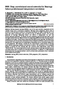
Fig.1 shows a snippet of time series extracted from BIDMC Congestive Heart Failure data set [16]. Each subsequence is extracted and labeled according to the dotted line by medical staffs. However, to acquire the well aligned and labeled data, it always needs great manual cost. N
0
N
N
N
N
1000
N V
N
N
2000
N
N
N
N
3000
Fig. 1 A snippet of time series which contains two types of heartbeat: normal (N) and ventricular fibrillation (V). a) b) c) d) 0
500
1000
1500
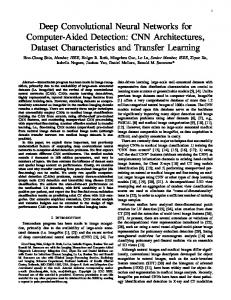
Fig. 2 Four 1D samples of 3D weakly labeled physical activities: a) ‘standing’, b) ‘walking’, c) ‘ascending stairs’, d) ‘descending stairs’.
In contrast to well aligned and labeled data, in practice, weakly labeled data can be obtained more easily [7, 15], which is defined as follows. Definition 5. Weakly labeled data: A long-term time series is associated with a single global label as shown in Fig.2. Due to the alignment-free property of weakly labeled data, it requires to extract subsequences by specific algorithm. The most widely used algorithm is sliding window [17], by which a large number of redundant subsequences may be extracted and all kinds of potential subsequences in alignment-free pattern space are covered. We illustrate the pseudo-code of sliding window algorithm in Algorithm 1. The parameters T , L and P denote the long-term time series, the window length and the sliding step. Supposing the length of T is n, it is easy to find that the number of extracted subsequences is d n−L+1 P e. In summary, in this paper, we will primarily concentrate on the time series of the same length and conduct experiments on both labeled data that is well aligned and weakly labeled.
Furthermore, for two multivariate time series X and Y, the Euclidean distance between them could be defined as follows: Xl ED(X, Y) = ED(xi , yi ) i=1
where l denotes the number of components, and xi and yi represent the ith univariate time series of them, respectively. As a simple measure, Euclidean distance suffers from several problems [2]. In the literature, DTW is considered as an alternative that is more robust than Euclidean distance and can align two sequences effectively [2, 9, 10]. To align two sequences (e.g., Q and C) using DTW, we need to construct a distance matrix first, which is shown as follows. d(q1 , c1 ) d(q1 , c2 ) · · · d(q1 , cn ) d(q2 , c1 ) d(q2 , c2 ) · · · d(q2 , cn ) .. .. .. .. . . . . d(qn , c1 ) d(qn , c2 ) · · · d(qn , cn ) Each element d(qi , c j ) of the matrix corresponds to the distance between the i-th point of Q and the j-th point of C, i.e., d(qi , c j ) = (qi − c j )2 . In this paper we primarily concentrate on the time series of the same length, thus we use two equal length time series to explain DTW for convenience. Notice that DTW can also be applied to time series with different length. A warping path W is a sequence of contiguous matrix elements which defines a mapping between Q and C: W = {w1 , w2 , ...wk , ..., w2n−1 }. Each element of W corresponds to a certain element of the distance matrix (i.e., wk = d(qi , c j )). There are three constraints that the warping path should satisfy, which are shown as follows. • Boundary : w1 = d(q1 , c1 ) and w2n−1 = d(qn , cn ). • Continuity: Given wk = d(qi , c j ) and wk−1 = d(qi0 , c j0 ), then i − i0 6 1 and j − j0 6 1. • Monotonicity: Given wk = d(qi , c j ) and wk−1 = d(qi0 , c j0 ), then i − i0 > 0 and j − j0 > 0. Since there may exist exponentially many warping paths, the aim of DTW is to find out the one which has the minimal warping cost: X2n−1 DTW(Q, C) = minimize wk W={w1 ,w2 ,...,w2n−1 }
k=1
4
Yi ZHENG et al. Exploiting Multi-Channels Deep Convolutional Neural Networks for Multivariate Time Series Classification
where W should satisfy these three constraints above. One step further, for two multivariate time series X and Y, similar to Euclidean distance, DTW between X and Y can be defined as follows: Xl DTW(X, Y) = DTW(xi , yi )
of CNN briefly and more details of CNN can be referred to [13, 21]. Then, we show the gradient-based learning of our model. After that, the related unsupervised pretraining is given at the end of this section.
where l denotes the number of components in multivariate time series, and both of xi and yi represent the ith univariate time series of them, respectively. It is common to apply dynamic programming to compute DTW(Q, C) (or DTW(X, Y)), which is very efficient and has a time complexity O(n2 ) in this context. However, when the size of data set grows large and the length of time series becomes long, it is very time consuming to compute DTW combined with k-NN method. Hence, to reduce the time consumption, window constraint DTW has been adopted widely instead of full DTW in many previous work [10, 18–20]. On the other hand, from the intuition, the warping path is unlikely to go very far from the diagonal of the distance matrix [10]. In other words, for any element wk = d(qi , c j ) in the warping path, the difference between i and j should not be too large. By limiting the warping path to a warping window, some previous work [10, 19] showed that relatively tight warping windows actually improve the classification accuracy. According to above discussions, we consider both Euclidean distance and window constraint DTW as the default distance measures in the following.
In contrast to image classification, the inputs of multivariate time series classification are multiple 1D subsequences but not 2D image pixels. We modify the traditional CNN and apply it to multivariate time series classification task in this way: We separate multivariate time series into univariate ones and perform feature learning on each univariate series individually, and then a traditional MLP is concatenated at the end of feature learning that is used to do the classification. To be understood easily, we illustrate the architecture of MCDCNN in Fig. 3. Specifically, this is an example of 2-stages MC-DCNN with pretraining for activity classification. Once the pretraining is completed, the initial weights of network are obtained. Then, the inputs of 3-channels are fed into a 2-stages feature extractor, which learns hierarchical features through filter, activation and pooling layers. At the end of feature extractor, the feature maps of each channel are flatten and combined as the input of subsequent MLP for classification. Note that in Fig. 3, the activation layer is embedded into filter layer in the form of non-linear operation on each feature map. We describe how each layer works in the following subsections.
i=1
3.1
3.1.1
3
Multi-Channels Deep Convolutional Neural Networks
In this section, we will introduce a deep learning framework for multivariate time series classification: MultiChannels Deep Convolutional Neural Networks (MCDCNN). Traditional Convolutional Neural Networks (CNN) usually include two parts. One is a feature extractor, which learns features from raw data automatically. The other is a trainable fully-connected MLP, which performs classification based on the learned features from the previous part. Generally, the feature extractor is composed of multiple similar stages, and each stage is made up of three cascading layers: filter layer, activation layer and pooling layer. The input and output of each layer are called feature maps [13]. In the previous work of CNN [13], the feature extractor usually contains one, two or three such 3-layers stages. For remainder of this section, we first introduce the components
Architecture
Filter Layer
The input of each filter is a univariate time series, which is l denoted xli ∈