Exploiting Non-Dedicated Resources for Cloud Computing Artur Andrzejak Zuse Institute Berlin (ZIB), Germany Email:
[email protected]
Derrick Kondo INRIA, France Email:
[email protected]
Abstract—Popular web services and applications such as Google Apps, DropBox, and Go.Pc introduce a wasteful imbalance of processing resources. Each host operated by a provider serves hundreds to thousands of users, treating their PCs as thin clients. Tapping the processing, storage and networking capacities of these non-dedicated resources promises to reduce the size of required hardware basis significantly. Consequently, it presents a noteworthy opportunity for service providers and operators of cloud computing infrastructures. We investigate how a mixture of dedicated (and so highly available) hosts and non-dedicated (and so highly volatile) hosts can be used to provision a processing tier of a large-scale web service. We discuss an operational model which guarantees long-term availability despite of host churn, and study multiple aspects necessary to implement it. These include: ranking of non-dedicated hosts according to their long-term availability behavior, short-term availability modeling of these hosts, and simulation of migration and group availability levels using realworld availability data from 10,000 non-dedicated hosts. We also study the tradeoff between a larger share of dedicated hosts vs. higher migration rate in terms of costs and SLA objectives. This yields an optimization approach where a service provider can find a suitable balance between costs and service quality. The experimental results show that it is possible to achieve a wide spectrum of such modes, ranging from 3.6 USD/hour to 5 USD/hour for a group of at least 50 hosts available with probability greater than 0.90.
highly volatile) hosts can be used to provision a processing tier of a web service. The non-dedicated hosts are assumed to be either privately-owned (by volunteers) or institutionallyowned commodity PCs with broadband Internet access. The restrictions on web services suitable for this scenario stem from the following factors: •
•
A non-dedicated host can go off-line (or become unavailable) at any time, without prior warning. An service must provide a sufficient level of redundancy and implement management mechanisms to mask such an outage. The transfer of data between non-dedicated hosts and other tiers (data center and Internet users) costs money. Furthermore, the bandwidth is usually limited (especially from the non-dedicated resources to other tiers). In effect, only moderate traffic rate can be supported by such hosts.
Despite these constraints there are a variety of suitable use cases: •
•
I. I NTRODUCTION Web applications and services such as Google Apps, DropBox, Go.Pc, and others are increasingly popular and require from their providers enormous computing resources. For example, the number of unique visitors to Google Docs and Spreadsheets has surpassed 1.4 million in October 2007 [1]. Simultaneously, the used client-server architecture introduces an imbalance: a host managed by a service provider serves hundreds to thousands of user PCs. Even worse, the latter are treated as thin clients even if their processing capacity might be similar to those of the servers. Tapping the processing, storage and networking capacities of these non-dedicated resources for provisioning of web services and applications already successful in the case of Skype, SETI@home and file sharing networks - promises to reduce the amount of required hardware basis by a two-digit factor [2]. Consequently, this approach presents a significant cost slashing opportunity (on the order of millions of USD) for service providers and operators of cloud computing infrastructures. In this paper we investigate how a mixture of dedicated (and so highly available) hosts and non-dedicated (and so
David P. Anderson UC Berkeley, USA Email:
[email protected]
•
• •
Bursting into the cloud, i.e. using (possibly internal) cloud computing resources to handle load spikes [3]. For example, Mars Inc. used Amazon’s EC2 to handle bursty traffic load during weekly candy giveaways. Certain Map-Reduce jobs, where the ratio of transferred data to computation on a map / reduce node is high, e.g. conversion of New York Times articles to pdf [4]. Personal storage applications (DropBox, Wuala). Here processing and data storage can be performed on nondedicated resources close to users, and backend file servers can be used in the worst case. Massively Multi-player Online Games where hosts coordinate players and check user scores by replaying [5]. Certain interactive applications like a personal mobile desktop (Go.Pc) or Google Docs. Such hosts can serve as a temporary backend assuming that sufficient redundancy is provided to avoid data loss.
Non-dedicated resources pose several security and privacy challenges which we silently delegate to research on virtualization and encryption techniques. We also assume that application-specific fault tolerance mechanisms (e.g. replication and map-reduce programming paradigm) shall transparently eliminate processing delays due to outages of nondedicated hosts. Even with these issues our approach presents a noteworthy opportunity; the scale of some services (100 000’s of dedicated hosts) make even moderate per-host savings very
n = # desired hosts d = # dedicated hosts
host replacement and data migration
initial data migration
N = # given hosts
selection of non-d. hosts
working set for interval i
i-th prediction interval (length pil in hours)
... ... ... ... ... ...
non-dedicated hosts
dedicated hosts
selection of replacements for failed non-d. hosts
Figure 1: Illustration of the resource provisioning process across many prediction intervals
significant as a total. Furthermore, companies have already started to use volunteer resources for cloud computing. The World Community Grid of IBM regularly runs short-lived batch jobs across volunteer resources. In this paper we propose and evaluate a set of techniques necessary to implement the above scenario. Specifically, the contributions of this study are the following: • We evaluate new and existing techniques for conducting short-term availability prediction of non-dedicated hosts. Our results show that for our data set (10,000 nondedicated hosts participating in the SETI@home project) the most practical solution is a combination of a very simple prediction approach combined with ranking of hosts according to their long-term availability behavior. • We derive an operational model that allows one to identify Pareto-optimal combinations of dedicated and shared hosts that optimize monetary costs or migration costs or both. This operational model is based on the prediction and ranking approaches. • Based on this model we study the trade-offs between a larger share of dedicated hosts vs. higher migration rate for a real-world data set to estimate the feasibility of the approach. Exemplary results show that for 50 hosts requested by a service provider, an allocation of 25 dedicated hosts out of 55 given will minimize total costs (disregarding the migration rate) at 3.60 USD / hour. An allocation 44 dedicated hosts out of 52 given will minimize the migration rate. Paper structure. In Section II we describe the overall assumptions and the operational model. Section III studies and evaluates prediction approaches. Section IV is devoted to the simulation of the operational model. Section V discusses related work. We conclude with Section VI. II. O PERATIONAL A SSUMPTIONS AND R ESOURCE P ROVISIONING M ODEL Most web services discern between processing hosts machines used for computation, not storing any permanent data - and data storage hosts which carry persistent data in form of DB’s and file systems. For example, in a typical 3tier web application, web and application servers are deployed on processing hosts while the DBMSs and file servers use
separate data storage hosts. Usually all data storage hosts require dedicated, high-available servers. In contrast, in many scenarios processing hosts can be dedicated or non-dedicated. In this work we focus on ensuring availability in mixtures of dedicated and non-dedicated resources used as processing hosts in a large web service. In principle, it would be possible to use only non-dedicated hosts. However, a small “core” set of dedicated resources reduces significantly the probability of a complete service breakdown. Moreover, the bandwidth of volunteers (in particular, the upload bandwidth) is too low to move all services to the volunteers themselves. A. Resource provisioning process The primary problem in our scenario are availability outages of non-dedicated resources: such processing hosts can become non-available and later available without any control of the service provider. Consequently, the traditional notion of (individual) availability needs to be a relaxed and subsumed by collective availability introduced in [6]. The latter is achieved if in a pool of N hosts at least n remain available over a specified period of time. If a service provider (i.e. resource receiver) requests from a cloud computing operator (termed resource operator) a set of n hosts, the resource operator will assign to him a working set of N ≥ n hosts with a necessary level of redundancy R = (N − n)/n ≥ 1. The working set hosts is composed of d dedicated hosts (selected as stated in Section III) and N − d non-dedicated hosts. To ensure an operation over a long time period the selection of the working set needs to be repeated periodically as illustrated in Figure 1. The time interval for which a working set is selected and operated is called the prediction interval. Its length (in hours) is designated as pil. At the end of each prediction interval hosts which dropped out need to be replaced by other (non-dedicated) hosts (selected as shown in Section III). These new hosts need to be initialized with working data which creates some migration costs. The selection and assignment of working sets is assumed to be done by central instance, but there are no inherent constraints to use a P2P or hierarchical architecture. B. Operational and SLA parameters In this section we outline how the parameters N , d are set (determining the size of the working set and number of
r(4) = r(3) = r(2) =
Computation of all Pareto-optimal combinations (N,d) for given n, ag, r
Computation of total costs tc and migration rate mr for each pair (N,d)
Provisioning process: N* = # of given hosts d*= # of dedicated hosts
r(1) = Monitoring of availability patterns in hosts
Host groupping by regularity rank r
SP requests ³ n hosts with availability guarantee ³ ag
SP chooses (N*,d*) by his constrains on migration and costs
Figure 2: Interaction between resource operator and service provider (SP) on operational and SLA parameters
dedicated resources in it, respectively). We also introduce several service quality metrics / specifications and discuss their interplay with N and d. Table I overviews the introduced symbols. Figure 2 illustrates the steps required to set the values of N and d for a resource request. In a preparatory phase we monitor availability of non-dedicated hosts over a period of several weeks. The recorded data is used to assign each host a regularity rank i defined in Section III-B. A lower i indicates that predictions are likely to be more accurate. We designate by r(i) a group of non-dedicated hosts whose rank is i. An initial provisioning request of a service provider must specify the number n of desired hosts and an availability guarantee ag, see Figure 2. The latter is defined as the probability that at least n of the hosts in the (possibly larger) working set remain available over time pil (i.e. this is a probability that the collective availability is achieved in a single prediction interval). For given r, n and ag we compute a representative set Z of Pareto-optimal combinations of N and d (see Section IV-D). Each pair (N, d) fulfills the availability guarantee ag and is Pareto-optimal in the sense that neither N nor d can be decreased (leaving the other parameter constant) without violating ag. We assume that hosts of lowest rank are used first, and only if these are exploited the next rank group is used. We evaluate here all ranks to compare them in terms of service quality and costs. For each Pareto-optimal pair (N, d) a larger d implies higher costs due to dedicated servers. On the other hand, larger d reduces the migration rate mr defined as the average number of failed (non-dedicated) hosts divided by N . The induced trade-off between higher costs vs. higher migration rate is slightly more complicated as we also need to consider that each replacement of a failed host (see Figure 1) incurs costs due to transfer of working data (i.e. migration costs). In Section IV-D we explain how the total cost tc (sum of the cost of the dedicated hosts and the migration costs) as well as the migration rate mr is computed for each optimal pair (N, d) under a given rank. In the final stage, we sort the pairs (N, d) according to the (increasing) total cost and according to the (increasing) migration rate. If a service provider has an upper bound on the total costs, he chooses a pair (N ∗ , d∗ ) with a total cost below just this threshold which minimizes the migration rate. An analogous approach is used if an upper bound on the migration
rate is specified. The selected combination (N ∗ , d∗ ) is then used in the resource provisioning process described in Section II-A. III. I DENTIFYING H OSTS WITH H IGH S HORT-T ERM AVAILABILITY Correct selection of non-dedicated hosts is the most essential step for providing high collective availability in each prediction interval (see Figure 1). In this section we propose several methods to achieve this task and evaluate them. A. Prediction scenario and approaches For each non-dedicated host we forecast its availability over the next prediction interval (see Figure 1). In other words, if t is the end of the last prediction interval, we want to predict whether or not a host will be available in the complete interval [t, t + pil] where pil is a multiple of an hour. The availability data per host is a string of bits, each representing non-availability (0) or availability (1) in a particular hour. The methods introduced in Sections III-A2 and III-A3 require a prediction model which is obtained by processing historical availability data in a training interval of specified length. The prediction results are evaluated on a test interval, a data segment following directly a training interval. To estimate the accuracy we use a prediction error defined as a ratio of mispredictions to all predictions made on the test interval (in case of our 0/1 data this corresponds to the popular Mean Squared Error, MSE). As availability patterns of hosts are likely to change over time, we recompute the prediction model after the end of each test interval. The complete prediction error of model-based predictors is computed over a succession of consecutive test intervals, with an updated model for each Symbol pil n N d ag mr tc r(i) Z
Definition prediction interval length desired number of hosts number of hosts given (working set) number of dedicated hosts availability guarantee migration rate total costs group of non-dedicated hosts with rank i Pareto-optimal combinations of N and d
Table I: Symbol definitions
1) Last value predictor: The last value predictor (abbreviated LastVal) is a simplistic predictor which uses the availability value in the last hourly interval before prediction (i.e. [t − 1, t], where t is in hours) as the prediction of availability for the interval [t, t+pil]. The advantages here are minimum computational cost and no need for model training (there is no model). 2) Classification-based predictors: Classifiers are wellstudied algorithms which create a function with a relation between its inputs and a discrete output similar to the one observed on the training data. A classifier is usually the most suitable predictor type if inputs and outputs are discrete [7] as in this case. We have tested several classifiers, including Naïve Bayes (abbreviated NB) [8], Support Vector Machine SMO (SMO) [9], K ∗ - an instance based classifier (K∗ ) [10], multinomial logistic regression model with a ridge estimator (Logistic) [11]. We have also initially used a C4.5 decision tree [12] but dropped it due to consistently bad accuracy in our case. The primary input to build a classification model is the availability value in the last hourly interval before prediction. Since this input does not exploit the power of classifiers to capture complex relationships, we have included additional information (features) per training and per test instance. These features were: • • •
time: time and calendar information of the last hourly interval before prediction at time t averages: averages of the host availability over the last 2, 4, 8, 16, . . ., 128 hours prior to the prediction time t switch ages: number of hours since last change of availability until the prediction time t.
3) Gaussian models of availability runs: This algorithm (abbreviated Gauss) models the lengths of both availability and non-availability runs (i.e. uninterrupted sequences of hourly availability or non-availability). To train a model we compute the average and standard deviation of the length of all availability runs in the training interval data (same for nonavailability runs) which allows us for modeling of run lengths by the Normal (Gaussian) distribution. To predict, we first compute the number k of hours since last switch. If the last observed state is availability, we compute the probability p that the end of prediction interval (i.e. k +pil) is still in the current availability run. If the last observed state is non-availability, we use the other Gaussian model to find out the probability p0 that k + 1 is in the current non-availability run (see Section III-A). A host is predicted as available (non-available) iff p ≥ 0.5 (iff p0 ≤ 0.5). Finally, if the standard deviation of a run length is above a specified threshold (separately for availability and nonavailability runs), we revert to the method from Section III-A1. This ensures that even if the run lengths are non-stationary predictions of a reasonable quality can be achieved.
0.25
Averaged prediction error (MSE)
one. We have implemented and evaluated three prediction approaches described in the following.
0.2
0.15
0.1
0.05
0
LastVal
NB
SMO
K*
Logistic
Gauss
Type of predictor
Figure 3: Average error of the prediction methods for pil = 1
B. Ranking of hosts Evaluation from Section III-D suggests that the accuracy of short-term predictions varies widely among non-dedicated hosts. To segregate these hosts we assign each of them a regularity rank i computed as follows. We first determine a host’s error score according to one of the two methods below. Then the hosts are sorted by decreasing error scores, and finally subdivided into groups r(1), . . . , r(4) of equal sizes corresponding to regularity rank values 1, . . . , 4. The computation of the error score is done as follows. a) MSE: Here we use the computationally cheap takelast predictor (Section III-A1) to perform predictions on the first part D of historical data (not used later). The MSE obtained in this way is used as the error score. b) Average number of availability switches: We exploit the result of [6] and use a metric called aveSwitches as the error score. It is defined as the number of changes between availability and non-availability (or vice versa) per week. C. Measurement method Data used throughout the paper has been gathered using the Berkeley Open Infrastructure for Network Computing (BOINC) [13] from hosts participating in SETI@home project. The BOINC client has been instrumented to record the start and stop times of CPU availability (independently of which application the BOINC local client scheduler chooses to run). It is important to note that these times of CPU availability are a subset of the times when a host was powered on, as the client would start or stop an interval depending on whether the machine was idle (the latter defined by the preferences of the BOINC client set by the user). On the other hand, availability does not imply that a host had an Internet connectivity at this time. For our studies we use the subset of 10,000 hosts chosen randomly from about 48,000 hosts that were actively running the client between December 1, 2007 and end of February 12, 2008. We assume that the CPU is either 100% available or 0% which is a good approximation of availability on real platforms.
0.25
D. Experimental evaluation
IV. F INDING O PERATIONAL PARAMETERS VIA S IMULATION
A. Method Table I overviews the symbols used in this section. We execute trace-driven simulations to determine the optimal costs and migration rates for each rank group. The simulated service runs continuously over the entire trace period (excluding the training data D). We vary the starting point of each simulated
0.2
Averaged prediction error (MSE)
Throughout this section we use the following settings and abbreviations. For model-based predictors, the first training interval had a length of 15 days (i.e. 15 ∗ 24 samples), and each subsequent one 30 days. We have updated the prediction model every 20 days. For explanation of the predictor types (LastVal, NB, SMO, K∗ , Logistic, Gauss) see Section III-A. For the predictor Gauss we found that the threshold to revert to the LastVal method of 4 works best. First, we evaluate accuracy of the introduced prediction techniques. Figure 3 illustrates for pil = 1 the MSE of each prediction algorithms averaged over 500 hosts selected randomly from our data set. The boxplot shows the lower quartile, median, and upper quartile values in the box; whiskers extend 1.5 times the interquartile range from the ends of the box while “crosses” outside them are considered outliers. As expected, we have a significantly larger error for longer prediction intervals (higher pil values). More surprisingly is that for pil = 1 simple predictors like LastVal and NB perform best. For pil = 4 the situation is very similar (figure omitted) but the best performing predictors are Gauss and again NB, with a smaller error variance of the latter. Subsequently, we study how additional features influence accuracy of classifier-based predictors. Figure 4 shows averages of MSEs (over 500 hosts as above, pil = 4) for such predictors and various features added one at a time to the base classifier input (see Section III-A2 for explanation of abbreviations). Except for SMO and time-based features, all errors are larger. Similarly, this holds for the case when pil = 1 (not shown). Our results show that sophisticated predictors do not have any consistent advantage over the extremely simplistic approach such as LastVal. This might be caused by the fact that only feature-scarce data is available for model training (essentially this data is just a bit string representing past availability), or that the host behavior is (on average) inherently non-predictable. On the other hand, ranking of hosts (Section III-B) has influence on the quality of predictions, as shown by experiments of Section IV. This indicates that hosts are stationary over time in having long or short uninterrupted sequences (runs) of availability. For hosts with long availability runs, the LastVal predictor works sufficiently well. Consequently, this prediction approach paired with host ranking is used in the following sections.
No features Time SwitchAge Averages
0.15
0.1
0.05
0
NB
SMO
K*
Logistic
Classifier type
Figure 4: Influence of the additional features for classifierbased prediction and pil = 4
service. So for a given pil of 1 or 4 hours, each simulation executes over 4000 and 2400 predictions respectively, ensuring statistical confidence in our results. The parameters for simulations are as follows. Hosts are ranked using the criteria of either average number of switches or MSE. We then simulate a minimum of 50 or 100 requested hosts (n). For each n, we vary the number of given hosts N (number of dedicated hosts plus the number of non-dedicated hosts) such that the redundancy varies from 1 (none) to 1.6. For each N , we vary the number of dedicated hosts allocated from 0 to n. We do this for pil’s of either 1 or 4 hours. B. Performance metrics We measure the performance results of each simulation with several metrics derived from the operational model (Section II). A particular business policy can weight each of these metrics accordingly. The first metric is the fraction of pil’s where the service provider was provided with at least n of the requested hosts. This reflects the collective availability level obtainable for each combination of dedicated and given hosts. The second metric is the total cost of achieving this service level. The total cost can be broken down into migration costs (to restart the service on a non-dedicated hosts at the start of a prediction interval), work costs (to transfer data to nondedicated hosts), and dedicated host costs. The third metric is the migration rate needed to achieve the service level. To compute the monetary costs, we assume that the cost of the dedicated host is 10 US cents per hour, which is equivalent to the hourly rate for a small instance on Amazon’s EC2. Amazon hosts one of the largest clouds and thus would be a candidate for our proposed hybrid approach. We assume that the cost to transfer data to non-dedicated hosts is 10 US cents per gigabyte. This is the cost charged by Amazon in the lowest tier for outgoing data transfers. Lastly, we assume that the amount of data transferred during migration from one nondedicated host to another is 10MB per hour. This is reasonable amount for relatively stateless application and web servers.
0.6 0.4 0.2 65
0.3
5
0.25 4
Migration rate
Cost for 50 hosts (USD/hour)
Fraction with at least 50 hosts
1 0.8
3 2
0.2 0.15 0.1 0.05
1
0 65
65 60 55 50
# given hosts (rank 1)
0
10
20
30
40
50
60 55
# of dedicated hosts
50
# given hosts (rank 1)
(a) Availability
0
20
10
50
40
30
60 55
# of dedicated hosts
50
# given hosts (rank 1)
(b) Total cost
0
10
20
40
30
50
# of dedicated hosts
(c) Migration rate
Figure 5: Performance and cost of MSE (n = 50, pil = 4, rank 1)
0.8 0.6 0.4 0.2
5
0.25
4
Migration rate
Cost for 50 hosts (USD/hour)
Fraction with at least 50 hosts
0.3 1
3 2
60 55 # given hosts (rank 4)
50 0
10
20
30
40
50
# of dedicated hosts
(a) Availability
0.1 0.05
1 65
0 65
0.2 0.15
60 55 # given hosts (rank 4)
50 0
10
20
30
40
50
# of dedicated hosts
0 65
40
60
55
# given hosts (rank 4)
(b) Total cost
20 50
0
# of dedicated hosts
(c) Migration rate
Figure 6: Performance and cost of MSE (n = 50, pil = 4, rank 4)
C. Results In the interest of space, we show only those results for rank 1 and 4. We find that that the availability guaranteed with MSE-based ranking is better than aveSwitches-based ranking by as much as 5% (see Section III-B for definitions). So we focus on the MSE-based results. In Figure 5, we show the availability guarantee, migration rate, and total cost for hosts in rank 1. Given a particular number of hosts N , we observe expectedly that the fraction of availability guarantees met decreases as the number of dedicated hosts decreases. When the number of given hosts N is equal to the minimum requested n, the fraction of availability guarantees met increases exponentially with an increase in the number of dedicated hosts. As the given number of hosts increases relative to the minimum requested, this rate of growth lessens to a linear rate with slope that approaches 0. The implication of this trend is that redundancy of even just a few percent can reduce greatly the fraction of dedicated hosts needed to achieve an availability guarantee. For example, increasing redundancy by 10% can improve the fraction of guarantees met by as much as 40%. In Figure 6, we show the availability guarantee, migration rate, and total cost for hosts in rank 4. Clearly, the fraction of availability guarantees met is significantly lower (by as much as 40%) than the fraction met for hosts in rank 1. The dependency on the fraction of availability guarantees met and redundancy is much stronger than for hosts of rank 1
due to high host unpredictability; the relationship is either exponential or linear with slope of 1. The implication is that we need as many as 3 times the number of non-dedicated hosts of rank 4 compared to the number of rank 1 in order to achieve the same rate of meeting the availability guarantee. We also determined the performance and cost trends when the minimum number of hosts requested is doubled to 100. From the simulations, we found that the migration rate for hosts of rank 1 only increases by a few percent to about 13% in comparison to the minimum requested of 50. Still, the total costs to receive a minimum of 100 hosts is roughly double that for 50 hosts; the cost of dedicated hosts is dominant. D. Optimizing costs We describe how the previous results can be used to determine cost optimal combinations of dedicated and given hosts. The plot shown in Figure 5 can be intersected with a horizontal plane (parallel to x-y) whose z-value is the availability guarantee ag. We then find curve Z with combinations of the number of dedicated hosts d and N . Then for each point in Z we have a total cost and the migration rate. We can then find two optimal points depending on: 1) popt_cost : minimal cost without considering migration rate 2) popt_mig : minimal migration rate. Applying the curve Z, a user can then decide on the optimal cost/migration combination. In Figure 7, we show the curve Z where the minimum availability guarantee is 0.90 with 50 hosts requested. Each line in this figure represents availability within some range
Availability level
0.98 0.96 0.94
Total cost wo migration (USD/hour)
1
Migration rate
Fraction of time available
0.25
0.90−0.93 0.93−0.96 0.96−1.00
5
0.90−0.93 0.93−0.96 0.96−1.00
Availability level
0.2
0.15
0.1
0.92 0.9
0.05
40
65
0.90−0.93 0.93−0.96 0.96−1.00
4.8 4.6 4.4 4.2 4 3.8
60
20 # of dedicated hosts
Availability level
0 50
55 0
50
55
60
65
3.6 50
55
(a) Pareto optimal for availability >0.90
60
65
# of hosts given
# of hosts given
# of given hosts (rank 1)
(b) Migration rate
(c) Total cost (excluding migration)
Figure 7: Pareto optimal for availability ≥ 0.90 of MSE (n = 50, pil = 4, rank 1)
Availability level
1
0.25
0.98 0.96 0.94
5
0.90−0.93 0.93−0.96 0.96−1.00
Total cost wo migration (USD/hour)
0.90−0.93 0.93−0.96 0.96−1.00
Migration rate
Fraction of time available
Availability level
0.2
0.15
0.1
0.92 0.9
0.05 40
65
4.8
0.90−0.93 0.93−0.96 0.96−1.00
4.6 4.4 4.2 4 3.8
60
20 # of dedicated hosts
Availability level
55 0
50
# of given hosts (rank 4)
(a) Pareto optimal for availability >0.90
0 50
55
60 # of hosts given
(b) Migration rate
65
3.6 50
55
60
65
# of hosts given
(c) Total cost (excluding migration)
Figure 8: Pareto optimal for availability ≥ 0.90 of MSE (n = 50, pil = 4, rank 4)
in particular [0.90,0.93), [0.93, 0.96), and [0.96, 1.00]. As expected, for a given number of hosts, availability increases with the fraction of dedicated hosts. Also, for a particular number of dedicated hosts, availability increases with an increase in number of given hosts, i.e., undedicated hosts. The reason that the lines in Figure 7 are not of equal length is because the availability level provided by a set of hosts tends to jump by increments of 0.03 or higher as the number of hosts in the working set is changed. Also in Figure 7, we show the line plots of the migration rate for each point of Z. We detail popt_cost and popt_mig for rank groups 1 and 4. For rank 1, the point that minimizes costs without considering migration rate is 25 dedicated hosts out of 55 given. The point that minimizes the migration rate is 44 dedicated hosts out of 52 given. For rank 4, the point that minimizes costs is 25 dedicated hosts out of 62 given hosts. The point that minimizes the migration rate is 49 dedicated hosts of 52 given hosts. These points can be used to guide a service provider toward the best operational configurations. V. R ELATED W ORK In cloud computing, the idea most related to our work is known as cloudbursting - dynamic deployment of a software application that runs on internal organizational compute resources to a public cloud to address a spike in demand [3]. Our work differs by considering non-dedicated, volatile
resources, and by an extensive study of availability issues, usually ignored in cloudbursting. The notion of collective availability for non-dedicated hosts only has been introduced in [6]. We exploit here this notion to develop a performance and monetary cost model for a hybrid system consisting of both dedicated and non-dedicated resources. The significant differences in this work to the model in [6] are that we consider also dedicated resources, use host ranking to achieve a service level, and deploy a cost model. There are several approaches for short-time predictions of host availability: 1) Statistical characterization of average availability, possibly with incorporation of calendar effects [14], [15], [16], [17]. Here statistics computed once are used for predictions. 2) Prediction of short-term availability using machine learning algorithms trained on historical availability [18], [19], [20], [21], [6]. 3) Clustering hosts according to their historical prediction accuracy, and using a simplistic model which projects the current availability state into short-term future. This approach is exploited in this paper in Section IV. The drawback of the first approach is that statistics such as average availability are too course for dynamic hosts. These statistics often do not capture the temporal structure of availability, and are often misleading in some cases due to
the following effects: • Hosts with relatively low average availability are possibly available for long time periods (e.g. weekends) - these would be ranked low but are still usable. • High availability does not help much if a host is switched on/off frequently and irregularly. The second approach partially resolves these deficiencies and has been used successfully in context of distributed systems, such as desktop Grids. In this work we compare in Section III classifier-based approaches and a domain-specific predictor (Section III-A3) against the third approach above. It turns out that - at least for the SETI@home data set - both the classifiers and domain-specific predictors are an “overkill” as their accuracy is not higher. VI. C ONCLUSIONS In this paper we showed how to make short-term availability predictions, and how long-term availability behavior of hosts could be leveraged to divide hosts into rank groups. We then applied these ranks groups in a performance and monetary cost model for meeting SLA’s in terms of availability guarantees. Specifically, our findings were as follows: • Prediction: predicting future availability using the last value work surprisingly well, especially combined with host ranking. By contrast, a domain-specific predictor based on a Normal model (Gauss) as well as classifierbased predictors under perform prediction using the most recent value. We also found that using MSE is the most effective way to divide hosts into rank groups (compared to average number of switches). • Operational model: we identify combinations of dedicated and shared hosts that optimize monetary costs or migration costs or both. This operational model is based on predictions, and ranking the hosts by their historical long-term availability patterns. For example, for 50 hosts requested from the rank group 1, an allocation of 25 dedicated hosts out of 55 given will minimize total costs (disregarding the migration rate) at 3.60USD / hour. An allocation 44 dedicated hosts out of 52 given will minimize the migration rate. Our future work will refine this approach along several dimensions. One of them is considering the capacity of individual hosts and not only host count as the measure of allocated resources. We will also study the impact of additional communication latency of volunteered resources. Another research target is the influence of migration on the application performance, and how to resolve it with asynchronous or live migration. A more advanced extension is to consider the geographic location of a host, which would require a new measurement method. We will also perform our study on a much larger data set collected over the recent two years and comprising more than 100k hosts. There remain several open questions related to cloud computing. Given appropriate data sets, our concept could be applied to a combination of machines from a private and public
clouds, and also to a mixture of commodity and highly reliable resources deployed in a single data center. We also do not deal in this work with any security / privacy issues, incentive schemes for volunteers, and consider only a single business aspect of cloud computing, i.e resource savings. VII. ACKNOWLEDGMENTS This research work is carried out in part under the ANR-funded Clouds@home project (ANR-09-JCJC-0056-01) and the EC-funded projects SELFMAN (FP6-034084) and eXtreemOS (FP6-033576), and by the National Science Foundation (OCI-0721124).
R EFERENCES [1] B. Bitzenhofer, “Google docs and spreadsheets.” http://blog.compete. com/2007/12/06/google-docs-spreadsheets/, Dec. 06 2007. [2] D. Kondo, B. Javadi, P. Malecot, F. Cappello, and D. P. Anderson, “Cost-benefit analysis of cloud computing versus desktop grids,” in 18th International Heterogeneity in Computing Workshop, (Rome, Italy), May 2009. [3] W. Fellows, “Rightscale rolls its on-ramp toward other cloud systems.” http://the451group.com/report_view/report_view.php?entity_id= 54321, Aug. 01 2008. [4] “Self-service, Prorated Super Computing Fun.” http://open.blogs. nytimes.com/2007/11/01/self-service-prorated-super-computing-fun. [5] “Cheat-resistant 3D IPhone game relies on score-checking replays.” http: //www.sciencedaily.com/releases/2009/07/090727204540.htm, 2009. [6] A. Andrzejak, D. Kondo, and D. P. Anderson, “Ensuring collective availability in volatile resource pools via forecasting,” in DSOM 2008, September 2008. [7] R. Vilalta, C. V. Apte, J. L. Hellerstein, S. Ma, and S. M. Weiss, “Predictive algorithms in the management of computer systems,” IBM Systems Journal, vol. 41, no. 3, pp. 461–474, 2002. [8] G. H. John and P. Langley, “Estimating continuous distributions in Bayesian classifiers,” in Proc. 11th Conference on Uncertainty in Artificial Intelligence, pp. 338–345, Morgan Kaufmann, 1995. [9] J. Platt, “Fast training of support vector machines using sequential minimal optimization,” in Advances in Kernel Methods — Support Vector Learning (B. Schölkopf, C. J. C. Burges, and A. J. Smola, eds.), (Cambridge, MA), pp. 185–208, MIT Press, 1999. [10] J. G. Cleary and L. E. Trigg, “K*: an instance-based learner using an entropic distance measure,” in Proc. 12th International Conference on Machine Learning, pp. 108–114, Morgan Kaufmann, 1995. [11] S. le Cessie and J. C. van Houwelingen, “Ridge estimators in logistic regression,” Applied Statistics, vol. 41, no. 1, pp. 191–201, 1992. [12] J. R. Quinlan, C4.5: Programs for Machine Learning. San Mateo, CA: Morgan Kaufmann, 1993. [13] D. P. Anderson, “BOINC: A system for public-resource computing and storage,” in 5th International Workshop on Grid Computing (GRID 2004), 8 November 2004, Pittsburgh, PA, USA, Proceedings (R. Buyya, ed.), pp. 4–10, IEEE Computer Society, 2004. [14] D. Kondo, A. Andrzejak, and D. P. Anderson, “On correlated availability in internet-distributed systems,” in 9th IEEE/ACM International Conference on Grid Computing (Grid 2008), (Tsukuba, Japan), September 29–October 1 2008. [15] W. Bolosky, J. Douceur, D. Ely, and M. Theimer, “Feasibility of a Serverless Distributed file System Deployed on an Existing Set of Desktop PCs,” in Proceedings of SIGMETRICS, 2000. [16] R. Bhagwan, S. Savage, and G. Voelker, “Understanding Availability,” in In Proceedings of IPTPS’03, 2003. [17] S. Saroiu, P. Gummadi, and S. Gribble, “A measurement study of peerto-peer file sharing systems,” in Proceedinsg of MMCN, January 2002. [18] J. W. Mickens and B. D. Noble, “Exploiting availability prediction in distributed systems,” in NSDI, USENIX, 2006. [19] P. Dinda, “A prediction-based real-time scheduling advisor,” in 16th International Parallel and Distributed Processing Symposium (IPDPS’02), p. 10, Apr. 2002. [20] R. Wolski, N. Spring, and J. Hayes, “Predicting the CPU Availability of Time-shared Unix Systems,” in Peoceedings of 8th IEEE High Performance Distributed Computing Conference (HPDC8), August 1999. [21] A. Andrzejak, P. Domingues, and L. Silva, “Predicting machine availabilities in desktop pools,” in IEEE/IFIP Network Operations & Management Symposium (NOMS 2006), (Vancouver, Canada), 2006.