Exploiting synchrony spectra and deep neural networks ... - IEEE Xplore

EXPLOITING SYNCHRONY SPECTRA AND DEEP NEURAL NETWORKS FOR NOISE-ROBUST AUTOMATIC SPEECH RECOGNITION Ning Ma, Ricard Marxer, Jon Barker and Guy J. Brown Department of Computer Science, University of Sheffield, Sheffield S1 4DP, UK {n.ma, r.marxer, j.p.barker, g.j.brown}@sheffield.ac.uk

ABSTRACT

al. [5] trained two long-short term memory (LSTM) RNNs for predicting speech and noise, respectively. The two source predictions were used to create a mask in order to suppress the noise regions in a noisy spectrum. To improve noise robustness of DNN-based ASR systems, additional features are often concatenated with conventional ASR features. For example, in noise-aware training (NAT) [6], crude estimate of noise spectra were used to augment noisy mel-spectrogram as input to the DNN-AMs. In [7] cochleagrams were combined with conventional spectrograms to improve ASR accuracy of a convolutional neural network based system. This paper presents a novel system that exploits deep neural networks (DNNs) and ‘synchrony spectra’ for robust automatic speech recognition in the context of the CHiME-3 challenge. The proposed synchrony spectra feature encodes pitch-related information and have been shown to be effective in the past for both pitch analysis and source separation [8], but have not been previously employed in ASR systems. In the current paper we explore their use at two points in a robust ASR system. First, as cues for speech detection in a DNN-based speech enhancement front-end. Second, as auxiliary features that can augment the conventional acoustic modeling features in the input to a DNN-based ASR system. The synchrony spectra features and the DNN system are described in detail in Section 2. Section 3 describes the evaluation framework and presents a number of systems. Section 4 presents speech recognition results and compares various techniques. Section 5 concludes the paper.

This paper presents a novel system that exploits synchrony spectra and deep neural networks (DNNs) for automatic speech recognition (ASR) in challenging noisy environments. Synchrony spectra measure the extent to which each frequency channel in an auditory model is entrained to a particular pitch period, and they are used together with F0 estimates either in a DNN for time-frequency (T-M) mask estimation or to augment the input features for a DNN-based ASR system. The proposed approach was evaluated in the context of the CHiME 3 Challenge. Our experiments show that the synchrony spectra features work best when augmenting the input features to the DNN-based ASR system. Compared to the CHiME-3 baseline system, our best system provides a word error rate (WER) reduction of more than 14% absolute and achieved a WER of 18.56% on the evaluation test set. Index Terms— Deep neural network, noise-robust automatic speech recognition, synchrony spectra, mask estimation 1. INTRODUCTION Applications of automatic speech recognition (ASR) technology are finally starting to become commonplace. Research on ASR has made substantial progress in the last few years, especially with the introduction of deep neural network (DNN) based acoustic modelling [1]. However, adverse acoustic environments, such as the presence of multiple sound sources and reverberation, remain a challenging task for many ASR systems. The CHiME-3 challenge [2] is designed to allow evaluation of modern speech recognition systems in such adverse conditions, by recording speech spoken in real noisy environments. There are many diverse techniques for noise-robust speech recognition. A popular class of methods is based on time-frequency (T-F) masking for speech separation. In such methods, estimated T-F masks can be used to enhance noisy speech, and the enhanced signals can then be directly used as input to a well-trained ASR backend. Deep neural networks have been used to predict such a T-F mask or clean speech features from a noisy signal. In [3] a two-stage mask estimation framework using deep neural networks was proposed. In the first stage, a separate neural network was used to predict a binary foreground/background assignment of each frequency channel in a spectro-temporal representation. In the second stage, a classifier (single-layer perceptron or support vector machine) was used to refine the prediction given the output from the first stage. In [4] a deep recurrent neural network (RNN) was proposed to predict clean speech features directly from noisy features. Weninger et

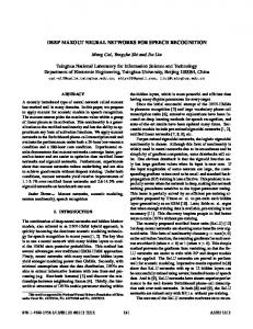
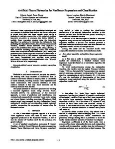
2. SYSTEM Figure 1 shows an overview of the two approaches described in the paper. The main contribution of the paper is the synchrony-spectradriven single-channel enhancement component. However, to evaluate single-channel enhancement in the context of the multi-channel CHiME-3 ASR task, we have integrated it into a system with a standard beamforming front-end (Section 2.4) and an ASR system based heavily on the CHiME reference system (Section 2.5). The single channel enhancement employs a deep neural network to estimate a time-frequency mask, which can then be used to filter out the interfering sounds. As input the DNN takes two types of feature: (i) features that encode the pitch and harmonicity of the target speech source, and (ii) features that are related to the presence of this pitch in each subband, i.e. the synchrony spectra (Section 2.1). The DNN is trained to map these features onto the probability that each time-frequency point is dominated by the target (Section 2.2). Beyond the enhancement stage, the synchrony spectra features can also be used as direct input to the DNN backend, where they are used to augment that standard acoustic features (Section 2.3).

This work was supported by the EU FP7 project TWO!EARS under grant agreement No. 618075

978-1-4799-7291-3/15/$31.00 ©2015 IEEE

490

ASRU 2015

by summing the ACG over all frequency channels, as follows:

SLWFKDQGV\QFKURQ\ VSHFWUXP FRPSXWDWLRQ

DXGLWRU\VSHFWURJUDP FRPSXWDWLRQ UDWHPDS

PDVNLQJ LPSXWDWLRQDQG VLJQDO UHFRQVWUXFWLRQ

S(τ, t) =

'11$65

'11PDVNHVWLPDWLRQ

EHDPIRUPHU

JDPPDWRQHÀOWHUEDQN

$6LQJOHFKDQQHOVSHHFKHQKDQFHPHQWDSSURDFK

Centre Frequency (Hz)

8K

Fig. 1: Two approaches described in the paper, both of which take their input from a beamformer front-end and are evaluated on the CHiME-3 challenge task. A: synchrony-spectra based singlechannel enhancement is used to derive an enhanced speech signal, which is passed to the DNN ASR backend for evaluation. B: conventional spectral features derived from a gammatone filterbank are augmented with pitch and synchrony spectrum features. The combined features are passed to the DNN ASR backend for evaluation.

g(i, t + k)w(k)g(i, t + k − τ )w(k − τ )

1370

440

1 0.8

The ‘synchrony spectra’ features describe the extent to which each frequency channel in the auditory model is entrained to a particular pitch period. These features are derived from the autocorrelogram (ACG), a model of auditory pitch estimation that combines both spectral and temporal information [9]. The ACG was computed as follows. An auditory front-end was employed to analyse the input signals with a bank of N = 32 overlapping Gammatone filters, with centre frequencies uniformly spaced on the equivalent rectangular bandwidth (ERB) scale between 50 Hz and 8 kHz [10]. Inner-hair-cell processing was approximated by half-wave rectification. Following this, the autocorrelation function of each channel was computed using overlapping frames with a shift of 10 ms. At a given time step t, the autocorrelation A(i, t, τ ) for channel i with a time lag τ is given by K−1

3600

50

2.1. Synchrony spectra

A(i, τ, t) =

(2)

The resulting ‘summary ACG’ S(τ, t) is shown in the bottom panel of Fig. 2. The position of the largest peak in the summary ACG corresponds to the pitch period of the strongest periodic sound source. '11$65

IHDWXUHFRPELQDWLRQ

JDPPDWRQHÀOWHUEDQN

EHDPIRUPHU

DXGLWRU\VSHFWURJUDP FRPSXWDWLRQ UDWHPDS

A(j, τ, t)

j=1

%)HDWXUHDXJPHQWDWLRQDSSURDFK SLWFKDQGV\QFKURQ\ VSHFWUXP FRPSXWDWLRQ

N

0.6 0.4 0

5

10

Autocorrelation Delay (ms)

15

20

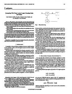
Fig. 2: Illustration of autocorrelogram and synchrony spectrum. The summary ACG is plotted in the bottom panel where the circle indicates the delay corresponding to the period of the fundamental. The rectangle shows the corresponding synchrony spectrum. The ‘synchrony spectrum’ is defined as the degree of synchrony to the period of the fundamental in each channel [8]. The fundamental of the strongest source was identified by selecting the largest peak in the summary ACG, corresponding to the lag τmax . The synchrony spectrum was then derived by sampling each channel of the ACF at τmax (as shown by the boxed region in Fig. 2). The resulting 32-D synchrony spectra were supplemented with the fundamental frequency (F 0) identified from the summary ACG and the pitch strength, which is the amount of periodic energy at the fundamental period normalised by the energy at lag zero, i.e., S(τmax , t)/S(0, t). This produces a 34-D vector of ACG features. The ACG features were used in two different ways in this study:

(1)

k=0

where g is the simulated hair-cell response and w is a Hann window of width K time steps. Here, we set K = 640 corresponding to a window width of 40 ms. The autocorrelation delay τ is computed from 0 to L−1 samples, where L = 320 corresponds to a maximum delay of 20 ms. The ACG is therefore defined as a three-dimensional volumetric function A(i, t, τ ), where the dimensions correspond to frequency channel (i), autocorrelation lag (τ ), and time step (t). Fig. 2 shows an example of a single correlogram frame (i.e., the value of A(i, t, τ ) at a specific time t) for an utterance from the CHiME-3 corpus. Most channels contain a peak at a lag corresponding to the pitch period of the sound, creating a characteristic ‘spine’ in the plot. In the example, the spine is centered on a lag of approximately 4 ms, corresponding to a fundamental frequency of 250 Hz. Since the autocorrelation function is periodic, similar spines also appear at multiples of this period. The pitch-related structure in the ACG can be emphasised

1. They were used to estimate a soft spectro-temporal mask that represents the probability of each time-frequency cell being dominated by the foreground speech. The mask was then used to synthesise the corresponding speech from the noisy mixtures (Fig. 1A). 2. They were used directly as supplementary ASR features to the DNN-based ASR backend (Fig. 1B). 2.2. Mask estimation with synchrony spectra We use a DNN to model the mapping between noisy speech features and a spectro-temporal mask. The learning target of the DNN is an

491

tional speech features with i-vectors capturing speaker identity [12] or with features characterizing the speech excitation signal [13]. It is unclear how the networks are exploiting these inputs, but it can be imagined that they are useful for normalising against some aspects of within-class variability. Motivated by these results, we have explored the use of synchrony spectra as auxiliary features that can be directly appended to the conventional ASR features being input into the DNN-based ASR back-end (approach B in Figure 1).

oracle mask that represents ideal foreground/background segregation. In the CHiME-3 data sets there exist both real data and simulated data. For the real data such oracle masks are difficult to obtain. However, for the simulated data we can compute oracle masks from the separate speech and noise signals that were used to create the simulated data. Hence, in this study the mask-estimation DNN is trained only on the simulated data. The instantaneous Hilbert envelope is computed at the output of each gammatone filter in the auditory front end. This is smoothed by a first-order low-pass filter with an 8 ms time constant, sampled at 10 ms intervals, and finally log-compressed to give an approximation to the auditory nerve firing rate – the ‘ratemap’ representation [11]. We then concatenate the 34-D ACG features with the 32-D ratemap features, producing a 66-D feature vector. The 66-D feature vectors were further spliced with the adjacent ±1 frames, forming a final 198-D feature vector as the input to the DNN. The DNN consists of an input layer, three hidden layers, and an output layer. The input layer contained 198 nodes and each node was assumed to be a Gaussian random variable with zero mean and unit variance. Therefore the 198-D feature input was Gaussian normalised before being fed into the DNN. The hidden layers had sigmoid activation functions, and each layer contained 1024 hidden nodes. The number of hidden nodes was heuristically selected. The output layer contained 32 nodes corresponding to the 32 frequency channels used in the auditory model. A sigmoid activation function was applied at the output layer. The neural net was initialised with a single hidden layer, and the number of hidden layers was gradually increased in later training phases. In each training phase, mini-batch gradient descent with a batch size of 256 was used, including a momentum term with the momentum rate set to 0.5. The initial learning rate was set to 0.05, which gradually decreased to 0.001 after 10 epochs. After the learning rate decreased to 0.001, it was held constant for a further 5 epochs. At the end of each training phase, an extra hidden layer was added before the output layer, and this training phase was repeated until the desired number of hidden layers was reached. The estimated T-F soft mask is then used to enhance the noisy signals by applying the mask to the gammatone filterbank output of the noisy signal, which is resynthesised using the overlap-add technique. Fig. 3 shows examples of enhanced signals using the ratemap representation as well as estimated masks. For comparison, the original noisy signal and the beamformed signal are also included in Fig. 3. Note that the synchrony spectra were measured at the fundamental of the strongest source (i.e. the biggest peak in the summary ACG). This makes the assumption that the strongest source will correspond to the target source in the mixture. This is typically a good assumption in the CHiME challenge data where the target talker is the closest source to the microphone and where the target has been enhanced by beamforming. In other situations the target pitch would have to be estimated more robustly, e.g. using a multipitch tracking algorithm.

2.4. The beamforming front-end The CHiME-3 challenge is a multimicrophone ASR challenge with 6 audio channels and is distributed with a minimum variance distortionless response (MVDR) beamformer enhancement baseline [2]. This baseline was reported to perform well on CHiME’s simulated test data but performed poorly on the CHiME real data set. Although reasons for the poor performance of the baseline are unclear, it was found that a substantial performance improvement could be obtained by replacing the front-end with the filter and sum beamformer implementation of Anguera et al. [14] which is freely distributed as the BeamformIt tool.1 This implementation was developed for robust meeting diarization and has a number of features not present in the CHiME baseline which might account for its superior performance, e.g. Wiener filtering of the channels prior to beamforming and post-processing of the TDOA estimates to filter out those that are unreliable. We applied the BeamformIt algorithm using its default configuration and using the five front-facing CHiME-3 microphones (channels 1 and 3–6). CHiME has a noisier rear-facing microphone (channel 2) which was found to be unhelpful and so was ignored. The output of the beamformer was then used as the single-channel input to the rest of the system (see Figure 1). 2.5. DNN backend We use the Time Delay Neural Network (TDNN) architecture and training procedure presented by Peddinti et al. [15] to estimate the HMM-state posteriors for each frame of the audio stream. In this architecture, each hidden layer takes as input the concatenation of the previous layer’s output at multiple time steps. The input layer of the network receives the LDA transformation of the feature stream spliced with two frames at each side. The neural network consists of six hidden layers. The indices of the time steps concatenated at each hidden layer are: -1, 2 for the second, -3, 3 for the third and -7, 2 for the fourth. A p-norm non-linearity is used for neurons activations [16], with p=2, an input dimension of 3500 and an output of 350. Finally a mix-up of 12000 was used for the final layer. The training strategy is similar to that employed for the mask estimation. Hidden layers are added gradually every two epochs. During each epoch a batch of 512 samples was used. The effective learning rate was gradually decreased from 0.0015 to 0.00015. The training consisted in 12 epochs. Training is performed in parallel using natural gradients and parameter averaging as described in [17] The LDA transformation and the DNN are trained using an alignment produced by the baseline GMM system. The frames at the input layer of the DNN are augmented with ivectors [12]. As in [15] the i-vector estimator was trained on a subset of the training set. Then i-vectors for the entire training set were estimated in an online fashion, with a history reset every two utterances. In order to increase i-vector variability and reduce the influence of

2.3. Synchrony spectra as auxiliary DNN-ASR features The synchrony spectra were primarily designed for supporting source segregation. The information they contain is related to pitch and would not traditionally be considered useful for phone classification. However, there have been several recent works showing that DNN-based ASR systems can take advantage of features that are only indirectly related to phonetic state. For example, performance improvements have been achieved by supplementing tradi-

1 See

492

http://www.xavieranguera.com/beamformit/

Noisy Ratemap

Noisy Ratemap

CF

8KHz

CF

8KHz

50Hz

50Hz

Beamformit Enhanced Ratemap


CF

8KHz

CF

8KHz

50Hz

50Hz

DNN Estimated Masks

DNN Estimated Masks

CF

8KHz

CF

8KHz

50Hz

50Hz

DNN Enhanced Ratemap


CF

8KHz

CF

8KHz

50Hz 0

0.5

1

1.5

2

2.5

3

Time [sec]

3.5

4

4.5

5

50Hz 0

5.5

0.5

1

1.5

2

2.5

3

(a) On the Bus

4

4.5

Time [sec]

5

5.5

6

6.5

7

7.5

(b) Cafe

Noisy Ratemap

Noisy Ratemap

CF

8KHz

CF

8KHz

3.5

50Hz

50Hz



CF

8KHz

CF

8KHz

50Hz

50Hz

DNN Estimated Masks

DNN Estimated Masks

CF

8KHz

CF

8KHz

50Hz

50Hz



CF

8KHz

CF

8KHz

50Hz 0

0.5

1

1.5

2

2.5

Time [sec]

3

3.5

4

50Hz 0

4.5

(c) Pedestrian Area

0.5

1

1.5

2

2.5

3

Time [sec]

3.5

4

4.5

5

(d) Street Junction

Fig. 3: Ratemaps representations of enhanced signals using various techniques. In each panel from top to right: original noisy signal; beamform-enhanced signal; DNN-estimated soft mask; Synthesised signal from the DNN-estimated mask. All signals are taken from the real data set of the CHiME 3 corpus.

environment noise, only utterances belonging to the same speaker and environment were paired together and considered as part of the same speaker. In the decoding stage the i-vectors are extracted on a per-utterance basis, one single i-vector is computed from the entire utterance and used for all of its frames. The setup and training procedure is readily available in the Kaldi toolkit [18].

made in four different noisy environments: ‘BUS’ – on a public bus; ‘CAF’– in a café’; ‘PED’ – a pedestrian area; ‘STR’ – a busy traffic intersection. Training data consist of 1600 real utterances collected from 4 speakers in the 4 environments, and 7138 simulated mixtures constructed by adding noise to the standard WSJ0 training set. The challenge provides separate development (dev) and evaluation (eval) test sets based on the original WSJ0 test sets, containing 330 × 4 and 410 × 4 utterances respectively, again with separate sets for real mixtures and simulated mixtures. The dev and eval sets each use four different talkers none of which appear in the training data.

3. EVALUATION The proposed systems have been evaluated using the data and rules of the CHiME-3 Challenge. A full description of the challenge is provided in [2] but essential details are summarised below for the sake of completeness. Training and test data come from recordings made by US-talkers speaking to tablet PC device fitted with six microphone around its frame. The data are WSJ0 sentences: either original recordings (‘Real’), or simulated mixtures made by adding clean recordings to separately recorded background noise (‘Simu’). Recordings are

The baseline systems include a GMM-based ASR system using MFCC features and a DNN-based ASR system using filter-bank features. In this study we employ the ratemap features obtained from the auditory front-end. 32 Gammatone filters were used for frequency analysis between 50 Hz and 8k Hz. The filter outputs were low-pass filtered and downsampled at 10 ms intervals. They were finally log-compressed to give an approximation to the auditory nerve firing rate.

493

nition in challenging noisy environments. Synchrony spectra are related to harmonicity of sound and they were used in this study either in a DNN for T-F mask estimation or to augment the input features for a DNN-based ASR system. The proposed approach was evaluated in the context of the CHiME-3 Challenge. Our experiments show that the synchrony spectra features work best when augmenting the input features to the DNN-based ASR system. Compared to the CHiME 3 baseline system, our proposed system provides a WER reduction of more than 14% absolute on the evaluation test set. The attempts to improve ASR performance using single-channel enhancement proved disappointing. Although the DNN was able to estimate masks that visibly reduced the noise in the T-F representation, this noise reduction did not translate into ASR gains. Note, beamforming by itself is already a very effective strategy for the CHiME-3 data and leaves little scope for further signal enhancement. It is possible that synchrony-spectra enhancement could be effective in single microphone systems where beamforming is not an option. The current study only evaluated the synchrony-spectra-based mask estimation in a GMM-based ASR system. In future we plan to feed the enhanced features directly to the DNN-based ASR or in combination with other ASR features. Another future direction is to tightly couple the mask estimation problem and speech recognition. Currently they are done in two separate DNNs. A more optimal way would be to combine the two in a unified DNN framework [19].

Discrete cosine transform (DCT) can be applied to the ratemap features for orthoganalisation, and this produces cepstral features similar to MFCCs. We refer to these cepstral features as GFCCs. The GMM-based ASR system employed the GFCC features. However, the DNN-based ASR system directly used the ratemap features. 4. RESULTS AND DISCUSSIONS Table 1 lists the word error rates (WERs) obtained by various systems evaluated in this study. First, results using the GMM-ASR backend are given at the top half of the table. For single channel noisy signals, our GMM baseline using the GFCC features achieved similar WERs to those of the MFCC baseline. The beamforming front-end using the 5 front channels substantially reduced the WER by on both the development set and the evaluation set. The DNN-based mask estimation was applied on top of the enhanced signals from the beamforming front-end. Although the DNN-enhanced signals show better signal-to-noise ratios (SNR) than the beamforming signals (Fig. 3), the masking technique improved very little over the beamforming signals. One explanation could be that the masking technique may introduce some distortions despite improving the SNR. In this study the system was simply retrained using the masked signals. Such distortions can sometimes degrade the performance of the acoustic models with retraining [19]. A better strategy would be to perform joint or adaptive training [20, 21]. The results using the DNN-based acoustic models were listed at the bottom half of Table 1. First, we show the result of our DNN backend using the same filter-bank features employed by the CHiME-3 DNN baseline. Our DNN system reduced WER on both the development set and the evaluation set, although larger improvement was achieved on the evaluation set (33.43% WER on reported by the CHiME-3 DNN baseline vs 29.61% WER achieved by our DNN system). All the other DNN-based systems included the development set during training. Compared to the GMM-based acoustic models, the DNN system reduced the WER by an average of 4% absolute on the evaluation test set. The beamforming frontend again substantially improved the performance by 7% absolute WER reduction on the evaluation set. Augmenting the ratemap features with the synchrony spectra features further reduced the WER of the beamforming DNN-based ASR system. The synchrony spectra features include F0 estimates and pitch strength. We further evaluated a system where the ratemap features were only augmented with these two features. This is our best performing system which scored 18.56% WER on the evaluation test set and is about 1% absolute WER reduction over the beamforming DNN system. It should be noted that with the full synchrony spectra features the total feature dimension of the input to the DNN-ASR system become 66-D, while with only the F0 features the feature dimension is 34-D. However, we did not re-tune the DNN system to handle the increased dimension. Overall the use of a beamforming frontend, the DNN backend and augmenting the recogniser features with F0 estimate provides an improvement of more than 14% in absolute WER over the baseline system on the evaluation test set.

6. REFERENCES [1] G. Hinton, L. Deng, D. Yu, G. Dahl, A.-R. Mohamed, N. Jaitly, A. W. Senior, V. Vanhoucke, P. Nguyen, T. Sainath, and B. Kingsbury, “Suppression of acoustic noise in speech using spectral subtraction,” Signal Processing Magazine, vol. 29, no. 6, pp. 82–97, 2012. [2] J. Barker, R. Marxer, E. Vincent, and S. Watanabe, “The third CHiME speech separation and recognition challenge: Dataset, task and baselines,” in Proc. IEEE 2015 Automatic Speech Recognition and Understanding Workshop (ASRU), 2015 (submitted). [3] A. Narayanan and D. Wang, “Ideal ratio mask estimation using deep neural networks for robust speech recognition,” in Proc. IEEE Int. Conf. Acoust., Speech, Signal Process. (ICASSP), 2013, pp. 7092–7096. [4] A. L. Maas, Q. V. Le, T. M. O’Neil, O. Vinyals, P. Nguyen, and A. Y. Ng, “Recurrent neural networks for noise reduction in robust ASR,” in Proc. INTERSPEECH-2012, 2012. [5] F. Weninger, F. Eyben, and B. Schuller, “Single-channel speech separation with memory-enhanced recurrent neural networks,” in Proc. IEEE Int. Conf. Acoust., Speech, Signal Process. (ICASSP), 2014, pp. 3709–3713. [6] M. L. Seltzer, D. Yu, and Y.-Q. Wang, “An investigation of deep neural networks for noise robust speech recognition,” in Proc. IEEE Int. Conf. Acoust., Speech, Signal Process. (ICASSP), Beijing, 2013, pp. 7398–7402. [7] A. Tjandra, S. Sakti, G. Neubig, T. Toda, M. Adriani, and S. Nakamura, “Combination of two-dimensional cochleogram and spectrogram features for deep learning-based ASR,” in Proc. IEEE Int. Conf. Acoust., Speech, Signal Process. (ICASSP), 2015, pp. 4525–4529.

5. CONCLUSIONS This paper presented a novel system that exploits synchrony spectra and deep neural networks for noise-robust automatic speech recog-

494

Table 1: Word error rates % achieved by various systems evaluated in this study. In the System column, the first line (e.g. ‘MFCC’) indicates ASR features and the second line (e.g. ‘Noisy’) indicates the input signal to the system. ‘Noisy’ here means the unprocessed signal from channel 5 that is used by the CHiME 3 baseline systems. ‘SyncSpec’ stands for Synchrony Spectra. In the Acoustic Model column, ‘Train Dev’ indicates that the development set was included during training. The best average WERs on the real data set are displayed in bold. System MFCC Noisy GFCC Noisy GFCC Beamform GFCC Beamform+Mask Fbank Noisy Ratemap Noisy Ratemap Beamform Ratemap + SyncSpec Beamform Ratemap + F0 Beamform

Acoustic model GMM GMM GMM GMM DNN DNN Train Dev DNN Train Dev DNN Train Dev DNN Train Dev

Mode Simu Real Simu Real Simu Real Simu Real Simu Real Simu Real Simu Real Simu Real Simu Real

BUS 18.57 25.67 18.07 26.91 12.98 17.05 13.67 17.13 14.66 22.64 8.78 17.47 5.96 8.56 5.63 8.61 5.62 7.85

Development Test Set CAF PED STR 22.01 14.76 16.59 17.76 13.03 17.86 21.06 14.79 17.95 18.53 13.51 18.80 18.13 12.54 17.35 13.35 10.21 14.57 18.07 13.67 17.45 13.73 10.86 13.58 18.13 12.17 13.70 14.62 11.37 15.47 8.89 3.72 3.50 8.85 5.03 6.55 7.46 3.19 3.61 6.25 3.42 5.32 7.01 3.14 3.79 5.66 3.48 5.63 6.96 3.22 3.50 5.81 3.20 5.19

Avg. 17.98 18.58 17.97 19.44 15.25 13.79 15.72 13.82 14.66 16.03 6.22 9.47 5.06 5.89 4.89 5.85 4.82 5.51

BUS 19.29 48.76 17.91 45.47 17.52 34.01 17.28 34.27 15.20 41.84 15.84 36.68 15.11 25.52 14.40 24.42 13.19 24.55

Evaluation Test Set CAF PED STR 24.71 22.58 20.90 33.84 28.18 21.74 23.57 22.02 21.33 33.04 27.52 21.89 24.58 25.76 26.20 22.75 22.44 16.75 24.58 25.85 26.26 22.43 22.59 16.59 21.09 19.22 17.69 31.81 25.99 18.83 23.07 20.81 19.80 30.58 23.60 17.56 23.66 24.08 23.63 20.62 17.97 14.01 23.55 22.11 22.69 18.43 17.99 14.68 22.95 22.15 21.83 18.42 16.87 14.42

Avg. 21.87 33.13 21.21 31.98 23.52 23.99 23.49 23.97 18.30 29.61 19.88 27.10 21.62 19.53 20.69 18.88 20.03 18.56

[18] D. Povey, A. Ghoshal, G. Boulianne, L. Burget, O. Glembek, N. Goel, M. Hannemann, P. Motlicek, Y. Qian, P. Schwarz, J. Silovsky, G. Stemmer, and K. Vesely, “The kaldi speech recognition toolkit,” in IEEE 2011 Workshop on Automatic Speech Recognition and Understanding. Dec. 2011, IEEE Signal Processing Society, IEEE Catalog No.: CFP11SRW-USB.

[8] P. Assmann and Q. Summerfield, “Modeling the perception of concurrent vowels: Vowels with different fundamental frequencies,” J. Acoust. Soc. Am., vol. 88, pp. 680–697, 1990. [9] M. Slaney and R. Lyon, “A perceptual pitch detector,” in Proc. IEEE Int. Conf. Acoust., Speech, Signal Process. (ICASSP), Albequerque, 1990, pp. 357–360. [10] B. Glasberg and B. Moore, “Derivation of auditory filter shapes from notched-noise data,” Hearing Res., vol. 47, pp. 103–138, 1990. [11] G. Brown and M. Cooke, “Computational auditory scene analysis,” Comput. Speech. Lang., vol. 8, pp. 297–336, 1994. [12] A. Senior and I. Lopez-Moreno, “Improving DNN speaker independence with i-vector inputs,” in Proc. IEEE Int. Conf. Acoust., Speech, Signal Process. (ICASSP), 2014. [13] T. Drugman, Y. Stylianou, L. Chen, X. Chen, and M. J. Gales, “Robust excitation-based features for automatic speech recognition,” in Proc. IEEE Int. Conf. Acoust., Speech, Signal Process. (ICASSP), 2015. [14] X. Anguera, C. Wooters, and J. Hernando, “Acoustic beamforming for speaker diarization of meetings,” Audio, Speech and Language Processing, IEEE Transactions on, vol. 15, no. 7, pp. 2011–2023, 2007. [15] V. Peddinti, D. Povey, and S. Khudanpur, “A time delay neural network architecture for efficient modeling of long temporal contexts,” in INTERSPEECH, 2015. [16] X. Zhang, J. Trmal, D. Povey, and S. Khudanpur, “Improving deep neural network acoustic models using generalized maxout networks,” in Proc. IEEE Int. Conf. Acoust., Speech, Signal Process. (ICASSP), 2014. [17] D. Povey, X. Zhang, and S. Khudanpur, “Parallel training of dnns with natural gradient and parameter averaging,” in ICLR 2015, submitted, arXiv:1410.7455v4 [cs.NE].

[19] A. Narayanan and D. Wang, “Joint noise adaptive training for robust automatic speech recognition,” in Proc. IEEE Int. Conf. Acoust., Speech, Signal Process. (ICASSP), 2014, pp. 2504– 2508. [20] H. Liao and M. J. F. Gales, “Adaptive training with joint uncertainty decoding for robust recognition of noisy data,” in Proc. IEEE Int. Conf. Acoust., Speech, Signal Process. (ICASSP), 2007, pp. 389–392. [21] O. Kalinli, M. L. Seltzer, and A. Acero, “Noise adaptive training using a vector taylor series approach for noise robust automatic speech recognition,” in Proc. IEEE Int. Conf. Acoust., Speech, Signal Process. (ICASSP), 2007, pp. 3825–3828.

495