Department of Mechanical Engineering, School of Engineering, University of .... vehicle comes to rest due to internal friction, aerodynamic drag and rolling ...... Tech. Tipler, P. A., & Mosca, G., 2007. Physics for scientists and engineers (Vol. 1).
Communications in Applied Sciences ISSN 2201-7372 Volume 1, Number 1, 2013, 135-160
Exploring Viable Methods of Evaluating and Computing Vehicular Drag and Rolling Friction Force Coefficients by Applying Principles of Geometric Similitude Sanwar A. Sunny Department of Mechanical Engineering, School of Engineering, University of Kansas, Lawrence KS 66045, USA
Abstract: The current study focuses on simple methods of quantifying vehicular drag and rolling resistance coefficients. It highlights the relationship between the drag coefficients (CD) of two m odels of varying scales but sharing g eometric and dynamic similitude and also describe a simple, small scale and low cost, yet comprehensive approach to quantifying the autom otive co efficient of Rolling Resistance or Friction (Crr), also known as the Rolling Resistance Coefficient (or RRC). Applying principles of fluid mechanics, especially Bernoulli’s law and by scaling models using Reynold’s Number (Re) and the Buckingham Pi Theorem at varying velocities u0, drag forces, the drag forces FD were supplem ented by conducting simple wind tunnel tests. Real drag analysis show a 10% deviation from the literature data, contributed to negligence of the governing flow equations of Navier Stokes, such as modeling principles relative to turbulence. Some com putational flow modeling principles were briefly discussed. For rolling friction coefficient method, coast down and dynamic speed trap tests of scaled models were conducted under varying body weighted conditions to converge on the value, where a high speed cam era monitored the m otion of the vehicle. The experim ent produced different equations of motion which were then solved analytically by num erical analysis techniques to com pute the rolling friction coefficient. Initial guesses in the least square optimization iterations provided coefficient values wh ere drag forces were normalized (Crr of 0.0116). Studies were com pared with literature and direct scaling abilities were attributed for quantifying the normalized value.
Keywords: Drag Coefficient, Rolling Friction Coefficient, Similitude, Wind Tunnel, Coast down
© Copyright 2013 the authors.
135
136
Communications in Applied Sciences
Introduction For years, the aerospace and automotive industries have been enhancing designs to lower the overall drag coefficient by streamlining the exterior panels and choosing different materials. Minimizing losses to drag and other external frictional forces, the vehicle requires less power to reach its relative peak. In other words, reducing certain parameters optimizes the overall vehicle fuel efficiency. Simple wind tunnels use elementary principles of fluid mechanics to study lift and drag forces on a solid body. A beam balance or strain gauge typically measures changes in elongation at the base of the body in a static setting. In most real analysis of drag forces, however, certain error is bound to occur for a complex body. This is especially true in the case of vehicles. Force fluctuations occur during the rotation of wheels when it is in direct contact with the ground. Although these differences are usually neglected in simplified experiments, they are crucial in understanding the behavior of a complex body. Computation Fluid Dynamics (CFD) software can successfully create a virtual setting with real parameters and considerations, thereby eliminating some errors to a degree. In recent years, the automotive industry has conducted research on finding and minimizing external forces hindering a car's motion. Better tire designs and threading
techniques
are
becoming
prevalent
design
considerations
as
manufacturers are now shifting focus from performance towards efficiency, striving to power more engine energy to the wheels and incurring lesser losses in the process. Almost always a dynamic testing approach is necessary for converging on the rolling friction coefficient. Coast down testing is a viable experiment conducted universally to observe the effects of rolling friction in moving bodies. In these tests, power from the engine is cut at a certain point, after which mostly external forces
Communications in Applied Sciences
137
work to slow down the body and ultimately bring the body to rest over a certain period of time. This distance and time period is then observed, monitored and numerically treated with fundamental vehicular motion laws of classical mechanics. With known parameters, advanced numerical analysis is then conducted on the results to find pertinent information key to the vehicle's performance. Although overall body mass is a great factor in reducing wheel friction, rolling resistance coefficient can be reduced to optimize a vehicle's performance and fuel efficiency (Ehsani et al 2009). In recent times, scientists and researchers have begun testing the automobile computationally to find important design parameters. The tests again include Computational Fluid Dynamics
studies for fluid flow around an
object (Hussain et al 2010) such as the vehicle exterior or even modeling and testing exterior panels using Finite Element Analysis (FEA) (Rimy and Faieza, 2010). Tires can also be constructed and tested to analyze the relationship between wheel design and the coefficient of rolling resistance in FEA with 2D and 3D modeling (Ze et al 2010) The present investigation, however, is to introduce a coast down technique which further utilizes a speed trap system by high speed imaging processes in a dynamic motion by a scaled model. Due to geometric similitude principles, a 1:10th scale model of a 1974 Model Volkswagen Super beetle will be used. Entry and exit points will be identified at which the vehicle will pass during two different separate points of time, and the time required to cover the distance in between will be numerically computed from video data. The overall body weight will be varied throughout the experiment to generate multiple equation models which will be solved analytically to zero in on the constant after utilizing elementary numerical least square optimization techniques. There exists other coast-down technique where speed and deceleration values in tests are effectively eliminated and is based on the time–distance function derived by new solution s of the coast-down equation that is free from speed and deceleration. This enables a considerable group of measurement error sources to be eliminated and the coast-
138
Communications in Applied Sciences
down technique sensitivity to be increased; so the small drag alterations due to the changes in vehicle aerodynamic configuration or tire parameters, such as load, inflation pressure and temperature, can be detected (Petrushov 1998). In this study, the real of drag forces will be highlighted, culminating in the measurement of the drag coefficient of a certain vehicle, the 1970s VW Super Beetle. Comparing results from available manufacturer’s literature, the reasons for inconsistencies can be observed. Principles of Similitude shall be applied to scale the actual full sized car down to a 1:10 scale model. Due to similarity in overall form, Reynolds Number (Re) will give the scaling factor for the effective velocities. The drag coefficient C D which is a directly proportional constant to drag forces can be reduced by minimizing the frontal area of a body and deflecting airflow away from sudden, sharp or hollow contours. Drag coefficient is the same for two bodies of exact shape, but different sizes. In other words, scaling does not affect a model’s coefficient of drag as long as the model and the full scale object are of the same exact shape. Pixelizations can be used to quantify the respective vehicles’ frontal area. Vehicle motion is caused by axle rotation which is in turn powered by the combustion in the automobile engine. As the power is cut from the source, the vehicle comes to rest due to internal friction, aerodynamic drag and rolling resistance at the wheels. The external frictional forces at the wheels are directly depended on the total vehicle weight, the traveling velocity and a proportional constant called the coefficient of rolling friction. This constant, denoted in this study as C rr, depends on the texture and structure of the road, vehicle weight and the wheel dimensions, among other factors. Frictional forces caused by air movement over the car are called drag forces. (Hibbeler 2007)
Experimental Design: Setup and Methodology
Communications in Applied Sciences
139
The vehicle body is first constructed for the drag test. A resin material is mixed under guided conditions and hardened at room temperature after letting it cure for 3 hours. Epoxy or polyepoxide, a thermosetting polymer is formed from the reaction of an epoxide "resin" with polyamine "hardener". As such, this epoxy is called the two part resin (the resin being a powder and the hardener being a liquid). This material will be applied to the model to provide a desired consistency and is very similar to the smoothness of convention sheet metal or fiber glass, which the vehicle exterior is made out of. Vacuum forming was initially used to produce a shell of the vehicle on which the material was poured. Finally, the model is secured to the wind chamber of a wind tunnel by a metal bracket (See Figure 1). An industrial fan provides air that travels over the static body. In principle, this effect is the equivalent of the body moving through the air. The air pushes on the body while traveling around the tested object causing drag forces from above and lift forces from below. The air flow then travels into a pipe and pushes fluids up the venture meter tube and fluctuates the fluid height (measured a s Δh). The elongation readings, caused by the flow of air on the body are sent to the control panel of a data acquisition software through a transducer. From these readings, corresponding drag forces are measured. Figure 2 shows the setup of equipment.
140
Communications in Applied Sciences
(a)
(b) Figure 1: a – b. Wind Tunnel Experimental Setup
Communications in Applied Sciences
141
Figure 2: Experimental Setup for speed trap tests For the rolling resistance tests, asphalt is chosen as the terrain for all the tests to imitate actual driving conditions for the coefficient. A scaled wireless model is used to run the tests. Due to principles of the Reynolds Number (Re) and Similitude, the following assumptions were made to extrapolate to full scale results. To scale the velocities for the car and the model, we use principles of geometric similitude by establishing a tenfold model to scale relationship. We can establish the relationship between the model and the full scale car by the respective Reynolds numbers. Hence,
uD uD s c a le d
where the vehicle fu ll
velocity ratio is given by u s c a le d u
fu ll
fu ll D fu ll s c a le d D s c a le d s c a le d fu ll
, or
u s c a le d 1 0 u
fu ll
;
This means that for the scaled model to experience the same magnitude of drag forces as
full scaled vehicle, the wind speeds it needs to run in would need to be
10 times the wind speed needed for the actual car.
142
Communications in Applied Sciences
The entrance and the exit point are spaced 103.5 inches (denoted in calculations as Xtrap ) away from each other. A 0.333 fps (frames per second) high definition camera was placed at the midpoint of the track to monitor the distances traveled with unit time. X1 and X2 refers to the exit first and second locations, while L2 and L1 refer to the entrance first and second locations respectively. SCcent and SCex were dimensionless scaling coefficients incorporated in the expressions to account for the discrepancies in measurements due to the spacing of the camera and the running track. See Figure 3. Entrance and exit velocities respectively were calculated as V ent
dx dt
X
2
X1
t fp s
and V e x
dl dt
L 2 L1 t fp s
(where
t fp s =
time lapse computed from the
camera frames) from where we say the mean velocity,
V
1 2
or
V0 t
V ex
V ent
from which the acceleration a,
was numerically computed with Δt being the time required for the car to completely clear the distance. The average acceleration
a
dv dt
V ex V ent t
(where t
X
tr a p
)
V
Mathematical Analysis Drag forces (F D) of a car are depended on
CD, the coefficient of drag for the
certain shape, ρ air, the mass density of the fluid through which the body is traveling, Afrontal or the vehicle’s effective frontal area and most importantly u, the mean velocity of the car. Afrontal is calculated both manually through photo pixelization and computationally through taking a section view and measuring the enclosed area in a 3d CAD software. The value of Afrontal was 0.0221 m2
Communications in Applied Sciences
143
(Sunny 2011a). Using the algorithms of the Pi Theorem, the drag forces which depend on the five above parameters; or
can be reduced using two
f x ( F D , u , A fr o n ta l , a ir , v 0 ) 0
dimensionless parameters culminating in the Reynolds number (Buckingham, 1914). Where
Re
u
A
and the Coefficient of Drag (C D) where
v
CD
FD 1 2
a ir A fr o n ta l u
2
Hence the function of five variables cane be effectively reduced by introducing a function of only two variables; where fy is some function of two arguments FD u A fy , 0 1 2 a ir A fr o n ta l u 2
Since drag force FD is the only unknown above, it is
possible to say FD 1 2
a ir A fr o n ta l u
2
u A fz
or
FD
u A 1 2 FD f z . a ir A fr o n ta l u 2
1 2
C D a ir A fr o n ta l u
and then
2
Historically, scientists and engineers, used various other methods to quantify the value using a velocity depended expression and a model that neglected the latter, i.e. it was not adjusted for velocity (Peck 1859). These expressions can be said to be F r o llin g C r r W c a r
which can be characterized for a slow rigid (minimum deformation)
wheel as: C rr
z d e p th
. A length dimension rolling friction coefficient was also introduced
d w heel
as F r o l l i n g
W car C rr rw h e e l
.
144
Communications in Applied Sciences
These simple models however were used before complex expressions were experimentally developed and do not directly correlate to recent data, but simply shows the relationships between the cars weight, the corresponding rolling frictional forces it experiences and the size of its wheels. It mainly leaves out any consideration for the travelling velocity. In effect, the rolling friction coefficient of a metal wheel of the same dimensions as a rubber wheel with equal loading and same rolling friction will give the same rolling resistance value. In this study, velocity was taken into consideration.
Then,
FS u p p lie d m t a
F ro llin g re s is ta n c e = C r r W V
(where
mt
was varied by
adding
weights) and also
(Crr is the coefficient of rolling resistance; which is depended on
wheel and road factors, among other conditions) where the weight,
W = mtg
; a
simplified force balance on the vehicle body showed
F FS u p p lie d F D ra g F R o llin g R e s is ta n c e
where
F D rag =
1 2
C D a i r A fr o n ta lV
2
This model is built on the assumption that during coastdown, drag and rolling friction forces are all that acts on the car. Another assumption pertaining to automotive drag would be neglecting any headwind or tailwind to the car. Total body weight was fluctuated with varying weights, to cause changes in friction forces thereby keeping drag forces relatively constant. Then numerical analysis techniques will then be used to converge on the coefficient of rolling resistance, by treating the drag coefficient as an unknown and then as neglecting it altogether given the low speeds of the speed trap tests. Lastly, drag coefficient of the same car was found experimentally from the wind tunnel analysis and was substituted to the simplified equations of motions during the tests. At coast down, i.e. when the engine is not providing power to the axles any longer, the body travels with the initial momentum and ultimately comes to a stop exclusively due to drag and friction forces slowing the car down, i.e the forces involved are, again:
Communications in Applied Sciences
F D rag =
1 2
C D a i r A fr o n ta lV
2
and
F ro llin g = C r r W c a r V
145
respectively. Both forces, FDrag and Frolling
are depended on the velocity of the travelling car. To fully quantify FDrag, the drag coefficient CD for the vehicle needs to be experimentally quantified, and any headwind or tailwind would produce an erroneous coefficient value if they are not added or subtracted from the velocity. Although at speeds traveled by the car during these speed trap tests, drag forces are effectively negligible. In any case, for better convergence on the coefficients of rolling friction, using drag coefficients would eliminate margins of error within the equations of motion (force balance and mechanics equations). The speed would be noted on the venture meter height readings or H (cm) and the changes in height (Δh) will correspond to changes in velocities u (mph). There exists a direct method of establishing a relationship between height readings and wind tunnel air speeds. It is now known universally as the Bernoulli’s Principle (Bernoulli 2004). The work-energy theorem can be used to derive Bernoulli’s principle (Tipler 2007). W Ek
i.e the change in the kinetic energy Ek of the system is equal to the net
work W done on the system; the velocity is hence derived as u
2 g h
or more specifically (Sunny 2011b), taking into account the fact that
the fluid is air, velocity is u
2SG g h
a ir
For drag considerations, in a real wind tunnel, the velocity u can be further treated with the decomposition technique as follows, denotes the time average of fluctuating
part, commonly
(often called the steady component), and known
as
where
u ( x , y , z , t ) u ( x , y , z ) u ( x , y , z , t )
u
perturbations. For stationary
the and
146
Communications in Applied Sciences
incompressible Newtonian fluids, the equations can be written in Einstein notation as:
u ju i x j
fi
u u j i p ij x x j xi j
u iu j
The properties of Reynolds operators are useful in the derivation of the RANS equations. Using these properties, the Navier–Stokes equations of motion, expressed in tensor notation, are (for an incompressible Newtonian fluid): ui xi
Hence:
0
ui t
u
ui j
x j
fi
1 p
xi
ui 2
x jx j
, Where fi is a vector representing
external forces. Each instantaneous quantity can be split into time-averaged and fluctuating components, and the resulting equation time-averaged, to yield: ui xi
0 牋so
ui t
ui
u
j
x j
u
j
ui
x j
fi
1 p
xi
ui 2
x jx j
Splitting each instantaneous quantity into its averaged and fluctuating components yields,
ui ui xi
0
or
ui ui t
uj u
Finally yielding
j
ui ui
u j ui x j
x j
fi
or
f
i
fi
1
p
p
xi
2
u
i
ui
x jx j
p 2 S u u ij ij i j x j
Another technique used for turbulence modeling is the Large Eddy Simulation (LES) Technique. LES is prevalent in a wide variety of engineering applications, including combustion, acoustics, and even simulations of the atmospheric boundary layer (Orszagt 1970, Yokokawa et. al 2002, Ehsani 2009) LES operates on the Navier-Stokes equations to reduce the range of length scales of the solution, reducing the computational cost. In mathematical Einstein notation, the Navier-Stokes equations for an incompressible fluid are:
Communications in Applied Sciences
ui xi
0
or
ui t
u iu x j
j
1 p
xi
147
ui 2
x jx j
The resulting sets of equations can be written as follows and are the LES equations: ui t
u
ui j
x j
1 p
xi
ui 2
x jx j
ij x j
The numerical solution of the Navier–Stokes equations for turbulent flow is very complex, and due to the significantly different mixing-length scales involved in the turbulent flow, the solution of this model requires such an extremely fine mesh resolution in which the computational time becomes significantly unrealistic (Orszagt 1970). Solutions to turbulent flow using a laminar solving technique usually result in a time-unsteady figure, which does not converge appropriately. CFD programs can be used to observe different fluid flow behaviors. See Figure 7. However, certain models such as the Reynolds-Averaged Navier Stokes Equations (RANS) in addition to utilizing turbulence models can be used in to maintain a level of accuracy in Computational programs. In addition, Large Eddy Simulation (LES) can numerically solve for the correct data, however it has economic limitation as it is an expensive computation tool and is financially not viable for virtual model testing. LES techniques, although meticulous and expensive than the RANS model has the ability to yield better results, since in it, larger turbulent scales are appropriately resolved (Yokokawa et. al 2002). Other turbulence models include the direct numerical simulation, Detached Eddy simulation and the Coherent vortex simulation. However, they are used for extremely complex models and recent developments allow for preconditioners that deliver mesh-independent convergence rates for any given system. These are beyond the scope of the current study and will neither be introduced nor discussed. A standard model known as SAE J1269 was developed by the Society of Automotive Engineers (SAE) to quantify the coefficient in the United States. C rr measured in
148
Communications in Applied Sciences
the study using the Force, Torque and Power methods denote the rolling resistance coefficient being measured as the proportion of energy that is lost to the hysteresis of the material as the tire rolls (Society of Automotive Engineers 2006). The study results of the general coefficient and its comparison to the applied forces at wheels are in agreement with (Lenard 2007). Another standard, SAE J2452 provided more accuracy for Crr value over a range of different vehicle loads (weight), tire pressures and vehicle speeds. as: C r r
P ? Z ?
a
The
model expression
bV cV
2
for the
standard is defined
Where P is the tire inflation pressure (in kPa or
psi), Z is the applied load for vehicle weight (in N or lbs), V is the vehicle speed (in km/h or mph) and α, β, a, b, c are the constant coefficients for the model (Society of Automotive Engineers 1999). In Europe, rolling resistance is tested using the standard ISO 8767 (International Organization for Standardization 1992). The SAE standard is similar to the patented C rr calculated methodoly of Hur et al 1997, where the distance time data during the coast down motion is effectively expressed. Applying Newton’s Second law of motion, or
W
(1 f )
g
dV dt
Where DT represent transmission loss, given by
DT D R D a
D T W ( 0 b V )
and DR, Da
represent Rolling friction loss and aerodynamic drag loss respectively denoted by (nI w I d ) g DR W kV 2 WR
Or
dV
a bV cV
2
2
and
where
g dt
Da C D
1 f
,
1 g V 2
2
F
a 0 f0
.
and c = k
CD F 2 g W
.
To obtain the velocity time data, the expression is integrated to yield d S (t ) dt
V (t )
gc
B ta n ( ta n
1
(
h B
) B (T t ) ) h
where S(t) is the distance travelled by
the vehicle from rest till t, T is the is the time from arbitrary t till stop.
Communications in Applied Sciences
Accordingly, B further
gA ,A 2
4ac b
integrated
to
2
and
h
gb 2
yield
1 h c o s ta n B S (T ) ln hT gc 1 h BT c o s ta n B
. Similarly, the expression can be
data
for
(t=T)
1 h c o s ta n B Tr B S (T i ) ln h Ti gc h 1 B (T r T i ) c o s ta n B
149
distance -time,
finally
we
i.e
have
where Ti is the time taken for the vehicle
to travel to the ith position in the speed trap. Again, h
f
gb 2
(nI w Id ) g WR
2
,
,
gb h0 0
0
,
B
(M Iw Id )g WR
2
,
gA 2
and
a 0 f0
A
4ac b
2
and finally
. Recalling that,
k
CD F 2 g W
1 f
.
Data results During the operational time period of 12 minutes, the following data were collected manually (venture meter tube heights and using the equation 3, the mean velocities) and automatically (Strain gauge data through transducer on the Labview software as Matlab data points converted to Drag Forces in Newton) for the drag test1.
Increasing Drag Coefficient (iCD) is 0.39 and Decreasing Drag Coefficient (dCD) is 0.41, With Full Scale Output (FSO) being 0.40 or 6.6% error within the tests according to the error, where: 1
iC D d C D % e r r o rh y s t FSO
100
,
150
Communications in Applied Sciences
0.50 0.45 Drag Coefficient
0.40 0.35 0.30 0.25 0.20 0.15 0.10 0.05 0.00 1 2 3 4 5 6 7 8 9 10 11 12 13 14 15 16 17 18 19 20 21 22 Test Figure 3: Drag Coefficients vs. Tests (Average Drag Coefficient, C D is 0.40) The actual drag coefficient of this model of the Volkswagen is 0.44 (Aird 2000), much higher than the results furnished by the wind tunnel (0.40 with a 10% error margin). An increased CD means that it is harder for the fluid to flow over the body. This difficulty can be contributed to the full scale car due to air flow causing disturbances underneath the car and at the wheels. The tested scaled model did not have wheels attached to it, nor was it resting on the ground. Moreover, external parts were taken off, such as side view mirrors and exhaust piping, all of which add blockades for the flow of air past the body. The actual CD data is produced under real parameters, much of which we considered insignificant during current tests. Ideal conditions were assumed and a few factors were negligible.
Communications in Applied Sciences
151
25
20
15
10
5
0 W (kg m/s2) Entrance V Exit V (mph) ΔV (mph) (mph) Trial 1
Trial 2
Trial 3
Δt (sec)
Acceleration (m/s2)
Average velocity (mph)
Trial 4
Figure 4 shows mean velocity and acceleration data from each of the weighted trials2. From the above data, we further quantify results into force components and solve numerically for Crr and CD. The below table shows both the first iteration conducted by a numerical analysis package (Least Square Linear Regression and Optimization Technique) utilizing a random initial guess, as well as the second and final iteration.
2
V 0 V ex V en t , where V ex and V e n t
are the mean set velocity readings from the 4 weighted test
run trials. W = m t*g where m t is the total vehicle mass and g is the gravitational acceleration constant.
152
Communications in Applied Sciences
Numerical
F supplied
Fdrag
F rolling
Iteration
mt. (ΔV 0/Δt)
Cd. α
Crr. β
Σ (F drag+
Δ |F supplied - Σ F d, R|
F rolling)
|mt. (ΔV 0/Δt)+( -Cd. α-
Cd. α+Crr. β
Crr. β)|
1
-7.115
-6.9125
-0.0075
-6.9225
0.6025
2
-7.1165
-6.262
-0.02175
-6.2825
1.1875
Table 1: Total forces acting on vehicle model and subsequent iterations Since
F 0 , Fs u p p lie d Fd ra g ? F ro llin g
at coast down; or
V0 mt t
-
1 2
C d a ir A f V V 0
2
C rr m t g V
Let
1 2
a ir A f V V 0
2
and
WV
where
W mt g
The above two iterations of least square methods yield a coefficient of rolling resistance of 0.1119 and then 0.3712, while the coefficient of aerodynamic drag yields 0.0416 and 0.1165, respectively. Other linear regression techniques such as Huber M, the least absolute deviations and nonparametric regressions but due to the analysis of simple non skewed and non-high tailed data distributions in Table 1, Least Squares optimization technique was preferred (Mohebbi et al., 2007). This analysis however were conducted assuming the coefficient of drag is a variable or an unknown, and an initial guess was selected to provide a starting point for the iterations, resulting in possibly erroneous end result. The same analysis was conducted by eliminating the drag coefficient, thereby only solving for the rolling friction constant, since at slow speeds, the drag coefficient is effectively negligible. Similarly knowing the drag coefficient for the model is 0.40, we can Fdrag into a constant, thereby solving for the Crr again as shown in Figure 5.
Communications in Applied Sciences
153
0.111 0.112
Fourth
0.098 0.099
Third
CD=0.4 0 0.113 0.114
Second
0.14 0.142
First
0
0.02
0.04
0.06
0.08
0.1
0.12
0.14
0.16
Figure 5: Coefficient of Rolling Resistance with CD= 0 and C D= 0.40 Knowing that the rolling resistance coefficient for a car the size of the test model would lie in between the ranges found assuming drag forces to be negligible (i.e. Fdrag~0.0 resulting in a Crr of 0.117) and the coefficient found after assuming that the model has a known constant drag coefficient found experimentally (i.e. Fdrag=C D*
1 2
a ir A f V V 0
2
, where CD is a constant of value 0.40; resulting in a Crr
of 0.115). The average coefficient of rolling resistance for the experiment therefore would be 0.116 where the mean Crr can be calculated as: C rr M
f rr ,C
D
K
f rr ,C
D
0
2
Where K is approaching the value of the coefficient of aerodynamic drag, i.e. less than or greater than CD ; Hence (K ≠ C D ); n is the total lines crossed, or more specifically, n is the exit position with n-1 the entrance position in the speed trap set up and M is the model-vehicle scale, moreover, f rr ,C
D
K
1 (X 2 t t fp s mt
n
X
n 1
L n L n 1 ) S C
n , n 1
1
C D A fr o n ta l S G h
154
Communications in Applied Sciences
(with the wind tunnel automotive drag force at varying tunnel air velocities of u0 where u0
2SG g h
where
a ir
or just 1 2
f rr ,C
D
a ir A f V V 0
K
2
and
1 (X 2 t t fp s mt
f rr ,C
D
0
n
X
n 1
L n L n 1 ) S C
1 (X 2 t t fp s mt
n
X
n 1
1
C D
n , n 1
L n L n 1 ) S C
n , n 1
This confirms findings from Ehsani et al. Since a 1:10 scaled model was used for this dynamic testing, the full scale vehicle velocity is given by V
s c a le d
V
fu ll
fu ll D fu ll s c a le d s c a le d D s c a le d fu ll
meaning V
s c a le
1 0 V
fu ll
,
where theoretical Crr for a full scale vehicle is given by 1 .6 0 9 C r r , th e o r e tic a l 0 .0 1 1 100
V
fu ll
,
However, it cannot be automatically used for a scaled model. Conversely, the velocity cannot be scaled up to that of a full sized vehicle and have the coefficients match between the scaled entities. Here in this study, we multiply the coefficient value with the scales since this test is conducted on a trap regardless of size, unlike the model by Ehsani et al 2009. This however results in higher error due to the precision of the tests, and negligence of the transmission losses. Still, the current study data on average comes within 0.005 of the patented results as shown in Figure 6 where
C rr , p
=10* C rr , p , sc a le d
Communications in Applied Sciences
Crr_bar
155
Crr, th, sc_bar
Crr, theory_bar 4
0.011
3
0.01
0.011216
0.012013
2
0.011
0.011465
0.012655
0.011472
0.014934
1
0.011198
0.014
0.011734
Figure 6: Test data comparison with literature and theoretical figures3 This scaling is independent of scaling factor incorporated due to Reynolds Number and similitude for the two velocities
V
themselves. Here
C rr
represents the
average experimental values of the coefficients with and without considering the effects of drag at given speeds
V scaled
(in mph). Knowing that
C rr , th e o ry
full scale vehicles, to scale down to the 1:10 ratio, we multiply the
is given for
C rr , th , sc
value by
10 to get data for the scaled model. The coefficient can be greatly changed by tire pressure, speed u or V, loading (curb weight W), wheel diameter and gap in data or measuring instruments, which is why most dynamic analysis do not directly correlate to literature data and result in errors as supported in (Wang 2004 et al). A slight change of the consistency of the ground material (concrete, sandy soil, loose soil, asphalt) changes the coefficient value dramatically (Wang 2003).
3
1 .6 0 9
V Where C r r , th , s c 0 .0 1 1 100
s c a le d
and C rr , th e o ry = 10 * C rr , th , sc due to scaling.
156
Communications in Applied Sciences
Recent Studies also show that C rr can range from a higher interval of 0.006 to 0.035 (Schmidt et al 2010) while the CD of the current model is, again, 0.44. This is in direct confirmation with the present study as the experimental range for the current study falls in this range; with, however, a high error of 43.416% for the mean values. Other studies conducted by the National Academy of Sciences, 2006, concluded that tires have a rolling resistance coefficient Crr of a range from 0.007 to 0.014 (or a 10.47% error in the mean values). Common values for the rolling resistance coefficient of a full sized vehicle travelling on concrete range from 0.010 to 0.015 (Gillespie 1992) or a mean of 0.0125. With respect to the current study, the this yields a 7.2% error. The average
C r r , th , s c
(Ehsani et al 2009) model values and
the Crr values of the study share a 2.31% error with each other. Although using the model-to-vehicle scaling ratio can be used to estimate the rolling friction coefficient for the actual vehicle, there are a lot of variables in such real life testing. To best optimize accuracy using this method, the curb weight for both the vehicles would need to be maintained, in addition to both overall exterior scale and tire dimensions. For coefficient of drag, the error is mostly attributed towards the failure of the computation tool to take all real world parameters into consideration during fluid flow analysis and solving governing flow equations (Navier-Stokes equations), such as modeling relative to turbulence (Acheson 1990). Most wind tunnel flows are usually simulated with the Navier Stokes Equation (Obayashi et. al 1998). Turbulence is a time dependent chaotic behavior seen often in many fluid flows (including air flows) caused due to the inertia of the fluid as a whole to the culmination of time dependent acceleration ; or flows where inertial behavior is insignificant and laminar. It is generally believed that the Navier–Stokes equations describe turbulence (Batchelor 1967).
Communications in Applied Sciences
157
Figure 7: CAD version of the study vehicle model in a CFD Add-on environment
Conclusions A reduction of drag forces significantly helps the cars efficiency (Sunny, S. A., 2013). Corrected design changes with verifiably lower coefficient of drag simply means that more energy will be going to the wheels of the car, as opposed to being used up in counteracting the drag forces that is exerted on the body by the air during motion (Ehsani 2009). This translates to more miles per unit volume of fuel, which in turn can mean lesser emissions given off by the car to travel the same distance. In most cases, the costs required to lower the drag coefficient pales in comparison to the fuel costs the car saves by being aerodynamically sound. Knowing rolling friction coefficient also has various applications in performance analysis and design of locomotives in everyday passenger car efficiency, as lower Crr tires could save 1.5–4.5% of all gasoline consumption (California Energy Commission 2003). It can even be important for more complex work such as correcting wheel sinkage during maneuvering through sandy terrains (Liu et al 2008) or even for misalignment correction by wheels aboard Microsatellites during
158
Communications in Applied Sciences
orbital maintenance (Si Mohammed et al., 2006). Better designs have led to reduced coefficient values at the wheels in cars (around 0.0025) such as Michelin Solar and Eco Marathon Cars (Roche et al). In normal passenger vehicles, energy is wasted by rolling frictions effects on the highways in which sound and heat is generated and given off to the surroundings as a by-product by the tires (Hogan 1973). Although industrial machines have been designed that have the ability to quantify the rolling friction coefficient of a tire, such equipment are usually not within the reach of most designers or scientists. This model is a small scaled and low cost technique that not only gives the scaled coefficient value with an acceptable degree of accuracy, but can be used to extrapolate the value to a full scaled car as long as weighted and scaled proportions, i.e. vehicle curb weight and tire size are the same. Certain common automotive designs save money on the fuel and provide more force to the drive train, meaning valuable supplied force will not be wasted on overcoming air friction and drag forces.
References Acheson, D. J., 1990. Elementary fluid dynamics. Oxford University Press, USA. Aird, F., 2000. Automotive Math Handbook. Motorbooks. Batchelor, G. K., 2000. An introduction to fluid dynamics. Cambridge university press. Bernoulli, D., J. Bernoulli
and J. Bernoulli, 2004.
Hydrodynamics and Hydraulics. Dover
Publications, New York. Buckingham, E., 1914. On physically similar systems; illustrations of the use of dimensional equations. Physical Review, 4(4), 345-376. California Energy Commission, 2003. California State Fuel-Efficient Tire Report: Volume I, Ehsani, M., Y. Gao and A. Emadi, 2009. Modern Electric, Hybrid Electric and Fuel Cell Vehicles: Fundamentals, Theory and Design. 2nd Edn., CRC Press, New York. Gillespie, T., 1992. Fundamentals of Vehicle Dynamics. 1 st Edn., Society of Automotive Engineers Inc., Warrendale, PA
Communications in Applied Sciences
159
Hibbeler, R.C., 2007. Engineering Mechanics: Statics and Dynamics. 11 th Edn., Prentice Hall Inc., USA., pp: 441–442 Hogan M. C., 1973. Analysis of Highway Noise, Journal of Soil, Air and Water Pollution, Springer Verlag Publishers, Netherlands, Volume 2, Number 3. Hur; N, I. Ahn and V A Petrushov. 1997. Method for measuring vehicle motion resistances using short distance coast-down test based on the distance-time data. U.S. Patent 5 686 651. Nov 11, 1997. Hussain, S.A., H.T. Tan and A. Idris, 2010. Numerical studies of fluid flow across a cosmo ball by Using CFD. J. Applied Sci., 10: 3384-3387. International Organization for Standardization, 1992. ISO 8767: Passenger car tyres - Methods of Measuring Rolling Resistance. TC 31/SC 3. ICS: 83.160.10 Lenard J. G., 2007 Primer on Flat Rolling. Elsevier Science. ISBN 9780080453194. pp 205. Liu, J., H. Gao and Z. Deng, 2008. Effect of straight grousers parameters on motion performance of small rigid wheel on loose sand. Inform. Technol. J., 7: 1125-1132. Mohebbi, M., K. Nourijelyani and H. Zeraati, 2007. A simulation study on robust alternatives of least squares regression. J. Applied Sci., 7: 3469-3476. National Academy of Sciences, Transportation Research Board, 2006. Tires and passenger vehicle fuel economy: Informing consumers, improving performance. Special Report 286., pp: 178 Obayashi, S., Fujii, K., & Gavali, S., 1988. Navier-Stokes simulation of wind-tunnel flow using LUADI factorization algorithm. Orszagt, S. A., 1970. Analytical theories of turbulence. J. Fluid Mech, 41(part 2), 363-386. Petrushov, V.A., 1998. Improvement in vehicle aerodynamic drag and rolling resistance determination from coast-down tests. Proceedings of the Institution of Mechanical Engineers, Part D: Journal of Automobile Engineering. Volume 212, Number 5. pp 369-380 ISSN: 20412991 Rimy, M.M. and A.A. Faieza, 2010. Simulation of car bumper material using finite element analysis. J. Software Eng., 4: 257-264. Roche, Schinkel, Storey, Humphris, Guelden, 1997. Speed of Light. ISBN 0 7334 1527 X Schmidt B, Ullidtz P, 2010 Special Report Danish Road Directorate and Dynatest. NCC Green Road: Energy savings in road transport as a function of the functional and structural properties of roads: A Technical Report.
160
Communications in Applied Sciences
Si Mohammed, A.M., M. Benyettou, S. Chouraqui, Y. Hashida and M.N. Sweeting, 2006. Wheel attitude cancellation thruster torque of LEO microsatellite during orbital maintenance. J. Applied Sci., 6: 2245-2250. Society of Automotive Engineers. 1999. SAE J2452 : Stepwise Coast down Methodology for Measuring Tire Rolling Resistance. SAE International Publications. Society of Automotive Engineers. 2006. SAE J1269 : Rolling Resistance Measurement Procedure for Passenger Car, Light Truck, and Highway Truck and Bus Tires. SAE International Publications. Sunny, S. A., 2011. Effect of turbulence in modeling the reduction of local drag forces in a computational automotive model. International Energy and Environment. 2(6):1079-1100. Sunny, S. A., 2011. Study of the Wind Tunnel Effect on the Drag Coefficient (CD) of a Scaled Static Vehicle Model Compared to a Full Scale Computational Fluid Dynamic Model. 4(3) : 236-245. Asian J of Sci Res. Sunny, S. A., 2013. The Convergence of Normalized Vehicular Rolling Friction Coefficient (Crr) by Dynamic High-Speed Imaging and Least Square Optimization Techniques. 3(3) : 609-625. British J. of Applied Sci. & Tech. Tipler, P. A., & Mosca, G., 2007. Physics for scientists and engineers (Vol. 1). Wh Freeman. Wang J, Dai J, Gao W, 2004. Application of Bench-based Rolling Resistance of Tires Model. Transactions of The Chinese Society of Agricultural Machinery Wang Q, 2003. A Calculation Method of the Sinkage and Rolling Resistance of a Rigid Wheel with Multi-Pass on Loose soil. Journal of Jilin University of Technology (Natural Science Edition) cnki: ISSN: 1671-5497.0.1987-03-011 Yokokawa, M., Itakura, K. I., Uno, A., Ishihara, T., & Kaneda, Y. (2002, November). 16.4-Tflops direct numerical simulation of turbulence by a Fourier spectral method on the Earth Simulator. In Supercomputing, ACM/IEEE 2002 Conference (pp. 50-50). IEEE. Ze P W, Qian X J, 2010. Simulation of Rolling Resistance of Tire Based on AN SYS. Journal of Advanced Materials Research (Volumes 156 – 157: Advanced Manufacturing Technology) pp 592-595. Doi: 10.4028/www.scientific.net/AMR.156-157.592