Jean-Michel Papy, Steve Vandenplas. Flanders' Mechatronics Technology Centre, Leuven, Belgium. Paul Sas and Hendrik Van Brussel. Katholieke Universiteit ...
Exponential Data Fitting for Features Extraction in Condition Monitoring of Paper-based Wet Clutches Agusmian P. Ompusunggu Katholieke Universiteit Leuven, Department of Mechanical Engineering, Division PMA, Leuven, Belgium
Jean-Michel Papy, Steve Vandenplas Flanders’ Mechatronics Technology Centre, Leuven, Belgium
Paul Sas and Hendrik Van Brussel Katholieke Universiteit Leuven, Department of Mechanical Engineering, Division PMA, Leuven, Belgium
ABSTRACT: Wet clutches play a critical role in automotive driveline systems as wet clutches may degrade while the driveline is running. Sudden failure of the running wet clutch causes unpredictable breakdown of the driveline. This is mainly due to friction material degradation. To avoid the latter, the friction material degradation history must be monitored. Unfortunately, such degradation is difficult to measure directly while the driveline is still running. Consequently, relevant features representing the friction material degradation level must be investigated. In this paper, damping ratio and torsional natural frequency at certain vibration modes are found to be relevant features. These are extracted with an exponential data fitting approach, wherein the free torsional vibration signal is modelled as a sum of exponentially damped sinusoids solved in a Total Least Squares (TLS) sense.
1 INTRODUCTION Wet clutches are widely used in many applications especially in the automotive field as devices to transmit mechanical power from the driving part to the driven part via a friction mechanism. Basically, a wet clutch consists of several friction and separator disks immersed in the automatic transmission fluid (ATF). For several decades, wet clutches with paper-based friction material have been used in many applications. It is well known that wet clutches play a critical role in automotive driveline systems. Obviously, wet clutches degrade while the driveline is running. The degradations occurring in a wetclutch are mainly caused by both friction material and ATF degradation. Those degradations are reported to deteriorate the friction characteristics of wet clutches (Ward et al. 1994). Several previous researchers, Gao et al. (2002) experimentally revealed that the Stribeck slope in sliding regime becomes more negative for degraded friction material than for new friction material. In contrast to the latter result, Li et al. (2003) revealed that the degradation of friction material has less impact on changing the Stribeck slope. Moreover, they also found that ATF degradation has a far greater impact than friction material degradation on changing the Stribeck slope to become more negative. Furthermore, due to friction material degradation, the topography of contact surface changes (Nyman et al. 2006). Quantitatively, the contact areas increase. This may lead to a change of the contact stiffness in so-called pre-sliding regime, corresponding to the post-engagement condition. Obviously, if this hypothesis holds, it implies that the modal parameters, such as torsional natural frequency and damping ratio also change. Remarkably, the latter parameters can be used as relevant features for monitoring the health condition of a wet clutch. In this work, a typical post-engagement torsional vibration signal, obtained from experimental data, is strongly transient and short, as depicted in Fig. 1a. Furthermore, Figs. 1b and 1c demonstrate that the main contribution lies in signal frequencies of less than 30 Hz. In this fre-
IOMAC'09 – 3rd International Operational Modal Analysis Conference
2
quency range, all frequencies are relatively constant. An appropriate method is obviously needed to extract the aforementioned modal parameters from such signal. In order to avoid uncertainties due to the inherent limitations of the discrete Fourier transform (Kay and Marple 1981) when applied to such short transient signal, a time-domain identification approach therefore was selected here.
Figure 1 : A representative torsional vibration captured post-engagement, (a) Signal in time domain, (b) Energy spectral density, and (c) Time-frequency map
In the time domain approach, identification of parameters from the aforementioned signal constitutes an exponential data fitting problem. This can be solved using either non-linear least squares minimisation or using a state-space approach. The first approach is an iterative method with possibly many local minima, so that the convergence is not guaranteed. In contrast, the second one is a non-iterative method. Although the latter approach is suboptimal, it nevertheless has a unique solution. There are several non-iterative time-domain methods commonly used in operational modal analysis, such as Ibrahim Time Domain (ITD) method and its variants (Mohanty and Rixen 2004). However, these methods may not be very robust to noise since signal and noise are well not separated. As a consideration, the Hankel Total Least Squares (HTLS) method was implemented because of its robustness and accuracy for estimating the parameters of such signals (Van Huffel 1993, Van Huffel et al 1994). 2 DESCRIPTION OF HTLS METHOD Principally, this method assumes that the stationary signal yn can be modelled as a sum of K exponentially damped complex values, sampled at uniformly distributed times tn = n.Ts, n = 0, 1,….,N – 1 (Papy 2005). K
K
i =1
i =1
y n = ∑ c i z in =∑ a i e jϕi e (− σi + j .ωdi )tn
n = 0,… ,N - 1
(1)
where j = − 1 , N is a number of data points, K is the model order, and Ts is the constant sampling period. The goal is to estimate the signal parameters such as damped natural frequencies ωdi, decaying factors σi, real amplitudes ai, and phases φi, i = 1, …,K. Furthermore, once the estimated signal parameters are obtained, the damping ratios can be determined. The HTLS is based on a state-space model of order K using N data points yn as formulated in Eq. (1) (Kung 1978) χ n+ 1 = Zχ n yn = Cχ n
(2)
3 where χn is a complex state vector, Z is the state-space system matrix, χ0 is the initial state vector, and C is the output matrix which are respectively expressed as follows: Z = diag ( z1 ,z2 ,… ,zi ) ∈
(3)
K ×K
χ 0 = [1,… ,1]
(4)
C = [c1 ,… , c K ]
(5)
T
Combining Eqs. (1) and (2) yields K
y n = CZ n χ 0 = ∑ ci z in
(6)
i =1
If matrices Z and C are obtained, then the signals parameters fdi, σi, ai, φi can be computed. But then, the question of how to compute these matrices requires a solution: First, the measured data points are arranged into a L x M Hankel data matrix H as follows ⎡ y0 ⎢ y H =⎢ 1 ⎢ ⎢ ⎣ y L −1
y 2 … y M −1 ⎤ ⎥ y 2 y3 … ⎥ ⎥ ⎥ … … … y N −1 ⎦ y1
(7)
with {L, M} selected such that N = L + M - 1 and L > K, and M > K. From Eqs. (1) - (7), this Hankel matrix can be directly decomposed into three matrices ⎡ 1 … 1 ⎤ ⎢ z 1 … z 1 ⎥ ⎡c K ⎥ ⎢ 1 ⎢ 1 H = ⎢ z12 … z K2 ⎥ ⎢ ⎥⎢ ⎢ ⎥ ⎢⎣ ⎢ ⎢⎣ z1L −1 z KL −1 ⎥⎦
0
0 ⎤⎥ ⎡1
z11
⎢ ⎥⎢ ⎥ 1 c K ⎥ ⎢⎣1 z K ⎦
z12 z
2 K
… z1M −1 ⎤ ⎥ T … ⎥ = SCT … z KM −1 ⎥⎦
(8)
Eq. (8) is well known as a Vandermonde Decomposition (VDMD), where the poles zi are also called generators. The column vectors of the S and T matrices are called Vandermonde vectors. It is obvious that using a Hankel data matrix and computing the VDMD of the Hankel matrix, the signal parameters can be easily derived. Computing VDMD is still possible (Boley et al 1994), but the non-orthogonality inherent in the Vandermonde vectors may lead to illconditioning. In general, obtaining parameters via orthogonal decomposition and subspace identification is numerically stable and robust to noise. Investigating Eq. (8) more thoroughly shows that the matrices S and T possess the “shiftinvariance” property that can be expressed as follows S↓ Z = S ↑
(9)
T↓ Z = T ↑
where the up and down arrows placed behind a matrix means delete the top or bottom row of the matrix, respectively. As is well known, Singular Value Decomposition (SVD) has a similar structure as Vandermonde decomposition. In addition, from the computational point of view, SVD is numerically stable. Performing SVD on Hankel matrix H yields ⎡ Σˆ H = Uˆ U 0 ⎢ ⎣0 LxL
[
]
0 ⎤ ⎡Vˆ H ⎤ ⎥⎢ ⎥ Σ 0 ⎦ ⎣V0H ⎦ LxM
MxM
(10)
IOMAC'09 – 3rd International Operational Modal Analysis Conference
4
where Uˆ ∈ LxK , U 0 ∈ Lx ( L − K ) , here Σˆ ∈ KxK contains the K non-zero singular values in decreasing order of magnitude, Σ 0 ∈ ( L − K ) x ( M − K ) , Vˆ ∈ MxK , V0 ∈ Kx ( M − K ) . Superscript H here denotes the Hermitian transpose. When the noise is absent in the signal, Σ0 is a null matrix and the SVD of H becomes the product of Uˆ Σˆ Vˆ H . On the other hand, when the signal is corrupted by noise, Σ0 is full rank. Note that the Vandermonde vectors (column vectors of S or T) span the same subspace as the Uˆ or Vˆ H columns. If a reasonable level of noise is present in the signal, then the truncated SVD of H ˆ ˆ ˆ ˆH H L× M = U L× K Σ K × K V M × K
(11)
ˆ which is the best rank-K approximation of H. H L× M can be considered as a denoised version of H even though it is no longer a Hankel matrix. Note here, the column vectors of Uˆ yield a good approximation of the subspace spanned by the Vandermonde vectors. In the noise-free case through using the similarity structure between SVD and VDMD, we conclude that Uˆ is equal to S up to multiplication by a square non-singular matrix Q ∈ K × K and can be mathematically expressed as follows Uˆ = SQ
(12)
Based on Eq. (12), the matrices Uˆ ↑ and Uˆ ↓ , which are deleted version of the top and bottom rows respectively, are related to the Vandermonde matrices S ↑ and S ↓ as expressed in the following mathematical formulation
Uˆ ↑ = S ↑ Q Uˆ ↓ = S ↓ Q
ˆ and combining Eq. (9) and (13) leads to the shift-invariance property of U ~ Uˆ ↑ = Uˆ ↓ Q −1 ZQ = Uˆ ↓ Z (U )
(13)
(14)
If this reasoning is also applied to the Vˆ ∗ matrix, this yields the shift-invariance property of Vˆ ∗ ↑ ~ Vˆ * = Vˆ * ↓ Z (V ) (15) ~ (U ) ~ (V ) * where the superscript denotes conjugation, while Z and Z are similar transformations of Z. In the presence of noise, the equalities expressed in Eqs. (14) and (15) no longer hold. In other words, the latter equations can be rewritten as ~ Uˆ ↓ Z (U ) ≈ Uˆ ↑ (16) ↑ ~ Vˆ * ↓ Z (V ) ≈ Vˆ *
(17)
Note that, Eqs. (16) and (17) are overdetermined, inconsistent, linear equations. These can only be solved using regression techniques. Here, these two are solved in the Total Least Squares (TLS) sense. Detailed explanation concerning TLS is fully described in Golub and Van Loan (1980). Otherwise, if they are solved in the Least Squares (LS) sense, then the method is called HSVD (Barkhuijsen ~ et al~. 1987). Once matrix Z (U ) or Z (V ) is obtained, then eigenvalue decomposition of the latter matrix is performed in order to obtain its eigenvalues λi which are the same with signal poles which is explicitly stated by Eq. (14)
λ i = ˆz i = exp{(− σ i + j 2πf di )Ts }
(18)
Note that the estimated signal pole is denoted by ˆz i instead of zi. Finally, the complex amplitudes ci can be estimated by solving an inconsistent set of equations
5
⎡ 1 ⎢ z1 ⎢ 1 ⎢ z12 ⎢ ⎢ ⎢⎣ z1N −1
1 ⎤ ⎡ y0 ⎤ c 1 ⎥ ⎡ 1 ⎤ … z K ⎥ ⎢ ⎥ ⎢⎢ y1 ⎥⎥ c2 … z K2 ⎥ ⎢ ⎥ = ⎢ y 2 ⎥ ⎥ ⎥⎢ ⎥ ⎢ ⎥ ⎢c ⎥ ⎢ ⎥ K … z KN −1 ⎥⎦ ⎣ ⎦ ⎢⎣ y N −1 ⎥⎦ …
(19)
in the LS sense. Once the complex amplitudes ci are obtained, then the real amplitudes (ai) and phases (φi) can be easily computed. Without prior knowledge of K, obviously, no reliable estimation of the signal poles is possible. Underestimation of K yields biased estimates, while overestimation will result in fitting the noise. Therefore, the determination of K is a key step in this method. In practice, K can be visually determined by observing either the number of dominant frequencies in the spectrum or number of significant singular values. Alternatively, there also exist several automatic model order selection methods (Badeau and Richard 2004, Quinlan 2007, Papy et al. 2007). 3 EXPERIMENTAL STUDY
3.1 Test setup A test setup was constructed in order to perform durability tests on a wet-clutch. Therefore, an accelerated life testing procedure is applied by increasing the energy level after every ten thousand clutch engagement cycles. The test is stopped when the friction material is considered to have completely failed. When testing, the clutch package is not immersed, but is sprayed by the ATF. The ATF is continuously filtered, such that it is reasonable to assume that the ATF used is not degraded during the service life. The experimental setup, depicted in Fig. 2, consists of three main systems: driveline, control, and measurement system. The driveline consists of seven components: input shaft, input flywheel, input electric motor for driving the input shaft, clutch package, output shaft, output electric motor, and output flywheel. Control systems are used for both controlling the input oil pressure to the clutch and for the speed control of input- and output-shaft. A multi-channel measurement system is used to measure all relevant dynamic signals.
Figure 2 : Experimental test setup.
IOMAC'09 – 3rd International Operational Modal Analysis Conference
6
The physical parameters measured during each clutch engagement cycle and their relevant sensors are listed in Table 1. No. 1 2 3 4 5
Table 1: Physical parameters measured Physical parameters Sensor Type Clutch pressure Piezoelectric pressure sensor Angular speed of input shaft Optical encoder Angular speed of output shaft Optical encoder Transmitted torque Optical electronic light sensor ATF temperature Thermocouple
Two electric motors with independent speed controllers are used as main drivers. Both motors are connected to the input and output shaft by a timing belt transmission. During start-up, the input electric motor drives the input shaft at a given rotational speed; simultaneously, the output electric motor independently drives the output shaft at the same rotational speed as the input shaft, but in the opposite direction.
3.2 Description of a clutch engagement cycle When the pressurized oil is applied into the clutch package at time tf (see Fig. 3), the clutch piston is activated, pushing the friction and separator disks towards each other. Consecutively, contact is established between separator and friction disks and the transmitted torque starts to build up at time te. The time between tf and te is called the filling phase. After the filling phase, the wet clutch enters the engagement phase. During this phase, the relative speed between input and output shaft decreases and the heat is dissipated by increasing the ATF temperature. The wet clutch is completely engaged when the relative speed reaches zero at time ts, hereafter called the engagement time. Some typical signals during a representative engagement cycle are shown in Fig. 3.
Figure 3 : Typical measured signals for one engagement recorded at 200th cycle
4 RESULTS AND DISCUSSION The torsional vibration signal captured post engagement, as depicted in Fig. 1a, is obtained from the torque sensor. The time-frequency map of this signal as shown in Fig. 1c is constructed using the Morlet wavelet transform. This is performed using the Open time-frequency toolbox (Auger et al. 1996). The stationary quality demonstrated by this map reveals that the signal with frequency contents of more than 30 Hz is strongly non-stationary. Since HTLS is valid for the
7 stationary signal, therefore, before applying this method for extracting features, the latter signal first needs to be filtered out. After applying HTLS to the filtered signal, two dominant frequencies appear, around 13 and 25 Hz. The model order is chosen manually at 8 (4 real sinusoids). According to the modal analysis results, the higher frequency of 25 Hz corresponds to the first torsional natural frequency of the driveline. Fig. 4 depicts the comparison between the analysed and the modelled signal using HTLS. From this figure, it is clear that both analysed and modelled signals match very well.
Figure 4 : Comparison between the actual and modelled signal
Obviously, a relevant feature is good if it shows a clear trend during the service life of wet clutches. Therefore, in order to investigate whether both damping ratio and torsional natural frequency can be used as features, the impact of these responsive parameters must be plotted. The latter parameters for the whole service life of the tested clutch are shown in Fig. 5. This figure shows that two dominant torsional natural frequencies in the beginning of the engagement cycles are relatively constant, and then they drop at certain number of engagement cycles. In addition, the damping ratio of each dominant frequency increases after the beginning of each engagement cycle; finally, they drop at certain number of engagement cycles (≈ 20,000th cycle).
Figure 5 : Torsional natural frequencies and damping ratios of two dominant frequencies for consecutive engagement cycles
8
IOMAC'09 – 3rd International Operational Modal Analysis Conference
5 CONCLUSIONS HTLS is a promising feature extracting method for condition health monitoring of wet clutches. Moreover, it is easy to implement. The two dominant torsional natural frequencies and damping ratios which are extracted by this method show a clear trend related to friction material degradation. Therefore, damping ratios and torsional natural frequencies can be used as relevant features for monitoring the degradation of wet clutches. REFERENCES Auger, F., Flandrin, P., Gonçalvès, P., Lemoine, O. 1996. Time-frequency toolbox: for use with Matlab. tutorial.pdf. [Online]. Available:http://tftb.nongnu.org/ Badeau, B.D.R. and Richard, G. 2004. Selecting the modeling order for the ESPRIT high resolution method: an alternative approach. In International Conference on Acoustics, Speech, and Signal Processing ICASSP04, volume II, p.1025–1028, Montr´eal, Qu´ebec, Canada, 17–21 May. Barkhuijsen, H., De Beer, R., and Van Ormondt, D. 1987. Improved algorithm for noniterative timedomain model fitting to exponentially damped magnetic resonance signals. Journal of Magnetic Resonance, p.73:553–557 Boley, D., Luk, F., and Vandevoorde. 1997. A general Vandermonde Factorization of a Hankel matrix. In Int. Lin. Alg. Soc. (ILAS) Symp. on Fast Algorithms for Control, Signals and Image Processing, Winnipeg. Gao, H., Barber, G.C., and Chu, H. 2002. Friction characteristics of a paper-based friction material, International Journal of Automotive technology, 3(4), p.171-176 Golub, G.H., Van Loan, C.F., 1980. An analysis of the total least square problem, SIAM J. on Numerical Analysis, 17(6), p.883-893. Kay, S.M. and Marple,Jr, S.L. 1981. Spectrum analysis-A modern approach. In Proceeding of the IEEE, 69(11). p.1380-1419. Kung, S.Y. 1978. A new identification and model reduction algorithm via singular value decomposition. Proc. 12th Asilomar Conf. on Circuits, Systems and Computers. Pacific Grove, CA, p. 705-714. Li, S., Devlin, M.T., Tersigni, S.H., Jao, T., Yatsunami, K., and Cameron, T.M. 2003. Fundamentals of Anti-shudder Durability: Part I-Clutch Plate Study, SAE paper No. 2003-01-1983. Mohanty, P. and Rixen, D.J. 2004. A modified Ibrahim time domain algorithm for operational modal analysis including harmonic excitation. J. of Sound and Vibration, 275 (1-2), p.375-390. Nyman, P., Maki, R., Olsson, R., Ganemi, B. 2006. Influence of surface topography on friction characteristics in wet clutch application. Wear, 261, p.46-52 Papy, J.-M. 2005. Subspace-based exponential data fitting using linear and multilinear algebra, PhD Thesis, K.U.Leuven Papy, J.-M., De Lathauwer, L., and Van Huffel, S. 2007. A shift invariance-based order-selection technique for exponential data modeling, IEEE signal processing letters. 14(7), p.473-476. Quinlan, A., Barbot, J.-P., Larzabal, P., and Haardt, M. 2007. Model order selection for short data: an exponential fitting test (EFT). EURASIP J. on Advances in Signal Processing. Article ID 71953. Van Huffel, S. 1993. Enhanced resolution based on minimum variance estimation and exponential modelling. Signal Processing, 33(3), p.333-335. Van Huffel, S., Chen, H., Decanniere, C., and Van Hecke, P. 1994. Algorithm for time-domain NMR data fitting based on Total Least squares. J. of Magnetic and Resonance, Series A 110, p.228-237 Ward, W.C., Sumiejski, J.L., Castanien, C.J., Tagliamonte, T.A., Schiferl, E.A., 1994. Friction and stickslip durability testing of ATF, SAE paper No. 941883