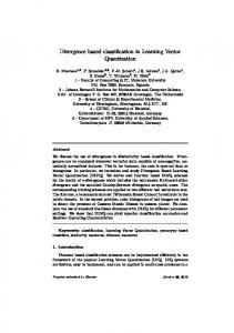
Extending Learning Vector Quantization for Classifying Data with Categorical Values Ning Chen1 and Nuno C. Marques2 1
GECAD, Instituto Superior de Engenharia do Porto, Instituto Politecnico do Porto, Rua Dr. Antonio Bernardino de Almeida, 431 4200-072 Porto, Portugal
[email protected] 2 CENTRIA/Departamento de Informatica, Faculdade de Ciencias e Tecnologia, Universidade Nova de Lisboa Quinta da Torre, 2829-516 Caparica, Portugal
[email protected]
Abstract. Learning vector quantization (LVQ) is a supervised neural network method applicable in non-linear separation problems and widely used for data classification. Existing LVQ algorithms are mostly focused on numerical data. This paper presents a batch type LVQ algorithm used for classifying data with categorical values. The batch learning rules make possible to construct the learning methodology for data in categorical nonvector spaces. Experiments on UCI data sets demonstrate the proposed algorithm is effective to improve the capability of standard LVQ to handle data with categorical values. Key words: learning vector quantization, self-organizing map, categorical value, batch learning
1
Introduction
Classification is of fundamental importance to solve many practical problems in a wide range of fields such as credit scoring, customer management, image segmentation, pattern recognition, medical diagnostics, and control systems. It can be regarded as a two-stage process, i.e., model construction from a set of labeled data and class specification according to the retrieved model. Kohonen’s learning vector quantization algorithm (LVQ) [1] is a supervised variant of the self-organizing map algorithm (SOM) that can be used for labeled input data. Both SOM and LVQ are based on neurons representing prototype vectors and use a nearest neighbor approach for clustering and classifying data. So, they are neural network approaches particularly useful for non-linear separation problems. In LVQ labels associated with input data are used for training. The learning process tends to perform the vector quantization starting with the definition of decision regions and repeatedly repositing the boundary to improve the quality of the classifier. Existing LVQ algorithms are mostly focused on numerical data. However, the categorical values are commonly seen in data sets and it is worthwhile to
2
Ning Chen and Nuno C. Marques
study the LVQ algorithm for classifying data with categorical values. In this paper, the idea of the proposed algorithm originates from NCSOM [2], a batch SOM algorithm based on a new distance measurement and update rules in order to extend the usage of standard SOMs to categorical data. In the present study, we advance the methodology of NCSOM to the batch type of learning vector quantization. We call this method BNCLVQ1 , an algorithm able to classify mixed numeric and categorical data. In one batch round, the Voronoi set of each map neuron is computed by projecting the input data to its best matching unit (BMU), then the prototype is updated according to incremental learning laws depending on class label and feature type. The main contribution of the proposed research is to extend the algorithms of LVQ family to handle data with categorical values for classification tasks. Experiments show that the algorithm outperforms standard LVQ with data preprocessing technique in terms of classification accuracy and achieves results as accurate as current state-of-the-art machine learning algorithms on various types of data sets. The remaining of this paper is organized as follows. Section 2 reviews the related work. Section 3 presents a batch LVQ algorithm to handle numeric and categorical data during model training. In section 4, we evaluate the algorithm on some data sets from UCI repository. Lastly, contributions and future improvements are discussed in section 5.
2
Related Work
2.1
Data Type and Distance Measurement
Data could be described by features in numeric and categorical (nominal or ordinal) types [2]. Nominal features are categorical taking on values from a limited and predetermined set of categories without natural ordering. Ordinal features have particular order but unknown distance. Let n be the number of input vectors, m the number of map units, and d the number of variables. Without loss of generality, we assume that the first p variables are numeric and the following d−p variables are categorical, {αk1 , αk2 . . . αknk } is the list of variant values of the k th categorical variable (the natural order is preserved for ordinal variables). In the following description, xi = [xi1 , . . . , xid ] denotes the ith input vector and mj = [mj1 , . . . , mjd ] the prototype vector associated with the j th neuron. Data projection is based on the distance between input vectors and prototypes using squared Euclidean distance on numeric variables and simple mismatch measurement on categorical variables [3]. d(xi , mj ) =
p X l=1
e(xil , mjl ) +
d X
δ(xil , mjl )
l=p+1
where
½ e(xil , mjl ) = (xil − mjl )2 , δ(xil , mjl ) =
1
0 xil = mjl 1 xil 6= mjl
Batch Numeric and Categorical Learning Vector Quantization.
(1)
Extending LVQ for Classifying Data with Categorical Values
3
This distance simply conjoins the usual Euclidean distance between numeric values with the number of agreements between categorical categories. Complementing [2], this paper will also present how to handle ordinal data in BNCLVQ. However care must be taken so that measures are compatible with the Euclidean values. 2.2
SOM Neural Networks
SOM is composed of a regular grid of neurons, usually in one or two dimensions for easy visualization. Each neuron is associated with a prototype or reference vector, representing the generalized model of input data. Due to its capabilities in data summarization and visualization, SOM is well suited for clustering, visualization and abstraction tasks [4]. Through a non-linear transformation, the data in high dimensional input space is projected to the low dimensional grid space while preserving the topology relations between input data. That is why resulting maps are sometimes called as topological maps. Normally, standard SOMs are applicable to numeric features through arithmetic operations on distance calculation and map evolution. NCSOM [2] is an extension of standard SOM to handle categorical data. It is performed in batch manner based on the distance measure in Equation (1) and novel updating rules. 2.3
LVQ Neural Networks
LVQ is a variant of SOM, trained in a supervised way in the sense that the classification information is included in model learning. The prototypes define the class regions corresponding to Voronoi sets. LVQ starts from a trained map with class label assignment to neurons and attempts to adjust the class regions according to labeled data. Several versions of LVQ are presented, e.g., LVQ1, LVQ2, LVQ3, batch LVQ, differing in the process of searching for the optimum boundaries of classes [1]. In the past decades, LVQ has attracted much attention because of its simplicity and efficiency. The classic online LVQs are studied in literature [5]. In these algorithms, the map units are assigned class labels in the initialization and then updated at each training step. The online LVQs are sequential and sensitive to the order of presentation of input data to the network classifier [1]. Some algorithms have been proposed to perform LVQ in a batch way [5]. E.g., a batch network algorithm FKLVQ [6] fuses the batch learning, fuzzy membership functions and kernel-induced distance measures. The batch type learning vector quantization is employed for tissue differentiation from magnetic resonance images [7], efficient image compression [8] and bankruptcy prediction [9]. LVQ is also a viable way to tune the SOM results for better classification and therefore useful in data mining tasks. In classification problems, SOM is firstly used to concentrate the data into a small set of representative prototypes with respect to the topology of input data, then LVQ is used to fine tune the SOM prototypes for best class separation. It was reported that LVQ is able to improve the classification accuracy of a usual SOM rather than a standalone method [10, 11].
4
Ning Chen and Nuno C. Marques
It is well known that LVQ is designed for metric vector spaces in its original formulation. Some efforts were conducted to apply LVQ to nonvector representations. For this purpose, two difficulties are considered: distance measurement and incremental learning laws. The batch manner makes possible to construct the learning methodology for data in nonvector spaces such as categorical data. The SOM and LVQ algorithms expressed in batch version are proposed for symbol strings based on the so-called redundant hash addressing method and generalized means or medians over a list of symbol strings [12]. Also, a particular kind of LVQ is designed for variable-length and feature sequences to fine tune the prototype sequences for optimal class separation [13]. In BCNLVQ, differently from the conventional approaches of data conversion in preprocessing phase, the categorical values are handled in the model learning. Due to the use of batch learning method and the close relation between SOM and LVQ, the presence of categorical values can be handled using the same strategy as NCSOM.
3
BNCLVQ: a Batch LVQ Algorithm for Numeric and Categorical Data
In this section, a batch LVQ algorithm for mixed numeric and categorical data will be given. Similar to NCSOM, it adopts the distance measure introduced in previous section. Before presenting the algorithm, we first define incremental learning rules that will be used in the proposed BNCLVQ algorithm. 3.1
Incremental Learning Rules
Batch LVQ uses the entire data for incremental learning in one batch round. During the training process, an input vector is projected to the best-matching unit, i.e., winner neuron with the closest reference vector. Following [1] a Voronoi set can be generated for each neuron, i.e., Vi = {xk | d(xk , mi ) ≤ d(xk , mj ), 1 ≤ k ≤ n, 1 ≤ j ≤ m} denotes the Voronoi set of mi . As a result, the input space is separated into a number of disjointed sets: {Vi , 1 ≤ i ≤ m}. At one training epoch, the Voronoi set is calculated for each map neuron, composed of positive examples (ViP ) and negative examples (ViN ) indicating the correctness of classifying. In Voronoi set an element is positive if its class label agrees with the map neuron, and negative otherwise. Positive examples fall into the decision regions represented by the corresponding prototype and consequently make the prototype move towards the input. While, negative examples fall into other decision regions and consequently make the prototype move away from the input. The map is updated by different strategies depending on the type of variables. The update rules combine the contribution of positive examples and suppress the influence of negative examples for each neuron in a batch round. Batch version is required for handling categorical values, since the number of values in neuron Voronoi set is used to define the weights. Assume mpk (t) is the value of the pth unit on the k th feature at epoch t. Let hip be the indicative function taking 1 as
Extending LVQ for Classifying Data with Categorical Values
5
the value if p is the winner neuron of xi , and 0 otherwise. Also, sip the denotation function whose value is 1 in case of positive example, and -1 otherwise. ( 1 if p = argmin d(xi , mj (t)) j hip = (2) 0 otherwise ½ 1 if label(mp ) = label(xi ) sip = −1 otherwise The update rule of reference vectors on numeric features conducts in the similar way as NCSOM. Since LVQ is used to tune the SOM result, here the neighborhood is ignored and the class label is taken into consideration. If the denominator is 0 or negative for some mpk , no updating is done. Thus, we have the learning rule on numeric variables: n X
mpk (t + 1) =
hip sip xik
i=1 n X
(3) hip sip
i=1
As mentioned above, the arithmetic operations are not applicable to categorical values. Intuitively, for each categorical variable, the category occurring most frequently in the Voronoi set of a neuron should be chosen as the new value for the next epoch. For this purpose, a set of counters is used to store the frequencies of variant values for each categorical variable, in a similar way to what was done for NCSOM algorithm. However, we have now taken into account the categorical information, so the frequency of a particular category is calculated by counting the number of positive occurrences minus the number of negative occurrences in the Voronoi set. F (αkr , mpk (t)) =
n X
v(hip sip | xik = αkr ), r = 1, 2, . . . , nk
(4)
i=1
F (αkr , mpk (t)) represents the accumulated absolute votes of each αkr value2 . As in standard LVQ algorithm, this change is made to better tune the original clusters acquired by SOM to the available supervised data. k For nominal features, the best category c = maxnr=1 F (αkr , mpk (t)), i.e., the value having maximal frequency, is accepted if the frequency is positive. Otherwise, the value remains unchanged. As a result, the learning rule on nominal variables is: ½ c if F (c, mpk (t)) > 0 mpk (t + 1) = (5) mpk (t) otherwise Different from nominal variables, the ordinal variables have specific ordering of values (here represented by index r). Therefore, the updating depends not 2
Function v(y | CON D) is y when CON D holds and zero otherwise.
6
Ning Chen and Nuno C. Marques
only on the frequency of values also on the ordering of values. The category closest to the weighted sum of relative frequencies on all possible categories is chosen as the new value concerning about the natural ordering of values. So, the learning rule on ordinal variables is: mpk (t + 1) = round( 3.2
nk X
F (αr , mpk (t)) r ∗ Pnk ) i=1 hip sip r=1
(6)
Algorithm Description
As mentioned, the BNCLVQ algorithm is performed in a batch mode. It starts from the trained map obtained in an unsupervised way, e.g., the NCSOM algorithm. Each map neuron is assigned by a class label with a labeling schema. In this paper the majority class is used based on the distance between prototypes and input for acquiring the labeled map. Afterwards, one instance xi is given as input and the distance between xi and prototypes is calculated using Equation (1), consequently the input is projected to the closest prototype. After all inputs are processed, the Voronoi set is computed for each neuron, composed of positive examples and negative examples. Then the prototypes are updated according to Equation (3), Equation (5) and Equation (6), respectively. This training process is repeated iteratively enough iterations until the termination condition is satisfied. The termination condition could be the number of iterations or a given threshold denoting the maximum distance between prototypes in previous and current iteration. In summary, the algorithm is performed as follows: 1. 2. 3. 4. 5.
4
Compute the trained and labeled map with prototypes: mi , i = 1, ..., m; For i = 1..., n, input instance xi and project xi to its BMU; For i = 1, ..., m, compute ViP and ViN for mi (t); For i = 1, ..., m, calculate the new prototype mi (t + 1) for next epoch; Repeat Step 2 to Step 4 until the termination condition is satisfied.
Empirical Analysis
The proposed BNCLVQ algorithm is implemented based on somtoolbox [14] in matlab running Windows XP operating system. In the empirical analysis, we mainly concern about the effectiveness of BNCLVQ in classification problems. 4.1
Data Sets
Eight UCI [15] data sets are chosen for the following reasons: missing data, class composition (binary class or multi-class), proportion of categorical values (pure categorical, pure numeric or mixed) and data size (from tens to thousands of instances). These data sets are described in Table 1, including the number of instances, the number of features (nu:numeric, no:nominal, or:ordinal), the number of categorical values (#val), the number of classes (#cla), percentage of instances in the most common class (mcc) and proportion of missing values (mv).
Extending LVQ for Classifying Data with Categorical Values
7
– soybean small data: a well-known soybean disease diagnosis data with pure categorical variables and multiple classes; – mushroom data: a large number of instances in pure categorical variables (some missing data); – tictactoe data: a pure categorical data encoding the board configurations of tic-tac-toe games, irrelevant features with high amount of interaction; – credit approval data: a good mixture of numeric features, nominal features with a small number of values and nominal features with a big number of values (some missing data); – heart disease: mixed numeric and categorical values (some missing data); – horse colic data: a high proportion of missing values, mixed numeric and categorical values; – zoo data: multiple classes, mixed numeric and categorical values; – iris data: pure numeric values.
Table 1. Description of data sets datasets soybean mushroom tictactoe credit heart horse zoo iris
#ins 47 8124 958 690 303 368 101 150
#features nu no or 0 35 0 0 22 0 0 9 0 6 9 0 5 2 6 7 15 0 1 15 0 4 0 0
#val 74 107 27 36 20 53 30 -
#cla 4 2 2 2 2 2 7 3
mcc 36% 52% 65% 56% 55% 63% 41% 33%
mv 0 1.4% 0 1.6% 1% 30% 0 0
To ensure all features have equal influence on distance, numeric features are normalized to unity range. The missing values contained in some data sets are neglected in the distance calculation and update operation of the corresponding features. 4.2
Experimental Results
In our experiments we set termination condition as 50 iterations. For each data set, the experiments are performed in the following way: 1. The data set is randomly divided into 10 folds. In each trail, 9 folds are used for model training and labeling, and the remaining is used for performance validation. 2. The map is trained with the training data set in an unsupervised manner by NCSOM algorithm, and then labeled by the majority class according to the known samples in a supervised manner. 3. BNCLVQ is applied to the resultant map in order to improve the classification quality.
8
Ning Chen and Nuno C. Marques
4. For validation, each sample of the test data set is compared to map units and assigned by the label of BMU. In order to avoid the assignment of an empty class, unlabeled units are discarded from classification. Then the performance is measured by classification accuracy, i.e., the percent of the observations classified correctly. 5. Ten-fold cross-validation is applied by repeating Step 2 to Step 4, while considering the different folds as test and training data and computing final average accuracy and standard deviation results.
Table 2. Effect of map size in classification accuracy datasets soybean mushroom tictactoe credit heart horse zoo iris
tiny(%) train test 100 100 92 91 73 75 85 83 86 80 83 81 82 81 95 97
small(%) train test 100 100 96 96 83 75 86 82 86 78 84 84 90 89 97 96
middle(%) train test 100 100 99 98 92 85 89 86 87 82 87 84 99 99 98 95
big(%) train test 100 100 99 98 95 84 92 85 88 79 90 81 100 96 99 95
Table 3. Average values of accuracy and standard deviation datasets soybean mushroom tictactoe credit heart horse zoo iris
map size [7 5] [14 8] [13 11] [17 7] [10 8] [11 8] [8 6] [16 3]
train accuracy(%) NCSOM BNCLVQ 100 ± 0 100 ± 2 96 ± 1 99 ± 1 80 ± 2 92 ± 1 85 ± 1 89 ± 1 87 ± 2 87 ± 2 83 ± 1 87 ± 1 99 ± 1 99 ± 1 98 ± 1 97 ± 1
test accuracy(%) NCSOM BNCLVQ 98 ± 8 100 ± 0 95 ± 4 98 ± 3 76 ± 3 85 ± 3 80 ± 4 86 ± 3 78 ± 9 82 ± 7 79 ± 10 84 ± 7 99 ± 3 99 ± 3 96 ± 3 95 ± 3
As other ANN models, LVQ is sensitive to some parameters in which map size, i.e., number of representative patterns, is an important one. In Table 2, we investigate the effect of map size to the resulted classification accuracy. Four kinds of maps are studied for comparison: ‘middle’ map is determined by the number of instances with the side lengths of grid as the ratio of two biggest eigenvalues [14]; ‘small’ map has one-quarter neurons of ‘middle’ one; ‘tiny’ map has half neurons of ‘small’ one; ‘big’ map has four times neurons of ‘middle’ one. As the map enlarges from ‘tiny’ to ‘middle’, both training accuracy and test accuracy improve significantly for most data sets (e.g., test accuracy increases
Extending LVQ for Classifying Data with Categorical Values
9
from 81% to 99% for zoo and 75% to 85% for tictactoe, while soybean and iris are less sensitive to the change of map size). Further enlarging the map increases the accuracy of training data, however, in case of test data, the accuracy has a tendency of getting downward, indicating the map becomes overfitting. It is shown that the maps in middle size are best for generalization performance except on iris data, which achieves desirable accuracy using only a ‘tiny’ map of 2 by 2 units. For simplicity, in the following experiments, we only report the results of maps in middle size. As summarized in Table 3, the results show the potential of BNCLQV compared with NCSOM in improving the accuracy on both training data and test data for not only data sets of pure categorical variables (e.g., soybean, mushroom and tictactoe) but also those of mixed variables (e.g., credit, heart, horse and zoo). Typically, BNCLVQ achieves increases up to 9% in classification accuracy, when comparing with using only NCSOM majority class for classification. The results where performance is almost equivalent are the soybean and iris data sets. In these datasets performance is already near reported maximum after running NCSOM3 . It is observed that performance on BNCLVQ networks is always better than the one of NCSOM on all datasets without overfitting maps. This gives evidence in favor of the validity of the approach for refining hybrid SOM maps. As mentioned previously, SOMs are very useful for data mining purposes. So, we have also analyzed our results from the visualization point of view. As an illustrative example we present the output map for credit data in Figure 1. Due to the topology preserving property of SOM, class regions are usually composed of neighboring prototypes of small u-distance (the average distance to its neighboring prototypes) values. The histogram of neurons contains the composition of patterns presented to the corresponding prototypes. Although neurons of zero-hit have no representative capability of patterns, they help to discover the boundary of class regions. From the visualization of u-distance and histogram, it becomes easy to obtain the visual insights into the cluster structures. Figure 1 shows the u-distance and histogram chart of trained map for credit data obtained by NCSOM (left graph) and BNCLVQ (right graph) respectively. Each node has an individual size proportional to its u-distance value with slices denoting the percentage of two classes contained. It is observed (by the zero-hit neurons) that BNCLVQ is able to separate two classes more clearly, showing the capability of BNCLVQ as a fine-tuning method of original NCSOM for better class discrimination. We also study the convergence properties of BNCLVQ algorithm on the data sets mentioned above. In this experiment, the convergence was measured as the overall distance inPprototypes between the current iteration and the previous m iteration: od(t) = i=1 d(mi (t − 1), mi (t)). As observed in Figure 2, the evolution of prototypes reflects the significant tendency of convergence. The distance decreases rapidly in the beginning, and tends to be more stable after a number 3
Indeed, as it was just verified in Table 2, in BNCLVQ the simpler iris dataset is presenting overfitting with the ‘middle’ map size (used for all datasets in this experiment).
10
Ning Chen and Nuno C. Marques
Fig. 1. Visualization of classification results on credit data.
of iterations (less than 50 iterations for these data sets). The convergence speed depends on the size of data, number of variables and intrinsic properties of data distribution. For example, it takes only 3 iterations to converge for soybean data. However for heart data, the variation of prototypes is not stable after 30 iterations due to the local optimum solution. As mentioned previously, overfitting is a critical problem for BNCLVQ as other ANN architectures. Indeed, according to our results, overfitting is already detected in some tested datasets. So, small improvements could be achieved with smaller maps or an earlier stop criterion. A practical approach to prevent overfitting is to use an independent validation data set to select the best model trained with different parameters, namely for defining the earlier stop in the training process. However, in this paper for the easier comparison among the methods discussed in next section, we have decided to use the conservative value of 50 iterations for assuring proper convergence of all maps. 4.3
Comparative Studies
For better comparison with other advanced approaches, the performance of proposed algorithm is compared with some representative algorithms for supervised learning. Six representatives implemented by Waikato Environment for Knowledge Analysis (WEKA) [16] with default parameters are under consideration: – Naive Bayes (NB): a well-known representative of statistical learning algorithm estimating the probability of each class based on the assumption of feature independence; – Sequential minimal optimization (SMO): a simple implementation of support vector machines (SVM). Multiple binary classifiers are generated to solve multi-class classification problems;
Extending LVQ for Classifying Data with Categorical Values
11
700 soybean mushroom tictactoe credit heart horse zoo iris
600
overall distance
500
400
300
200
100
0
0
10
20 30 number of iterations
40
50
Fig. 2. Convergence study of BNCLVQ.
– K-nearest neighbors (KNN): an instance-based learning algorithm classifying an unknown pattern to the its nearest neighbors in training data based on a distance metric (the value of k was determined between 1 and 5 by crossvalidation evaluation); – J4.84 : the decision tree algorithm to first infer a tree structure adapted well to training data then prune the tree to avoid overfitting; – PART: a rule-based learning algorithm to infer rules from a partial decision tree; – Multi-layer perceptron (MLP): a supervised artificial neural network with back propagation to explore non-linear patterns. We should stress that this comparison may be unfair to LVQ. Indeed, as discussed, LVQ is mainly a projection method that can also be used for classification purposes. So, for the sake of comparison, the standard LVQ is also tested. For doing so, categorical data are preprocessed by translating each categorical feature to multiple binary features (i.e., the standard approach for applying LVQ to categorical data). The summary of results is given in Table 4. For each data set, the best accuracy is emphasized by bold. Although BNCLVQ is not the best one for all data sets, it produces desirable accuracy in most cases, and reported best values are always within standard deviation (deviation values are reported in Table 3). Results are especially relevant on data of mixed types. Also, BNCLVQ is always better than standard LVQ, the only exception on tictactoe data is probably caused by the presence of interaction between features [17]. Indeed in tictactoe, other tested algorithms with categorical features (e.g. J4.8 and PART) had systematically worst performances. Maybe the inclusion of extra 4
A Java implementation of popular C4.5 algorithm.
12
Ning Chen and Nuno C. Marques
variables is somehow helping generalization and showing the need for better feature encoding. E.g., in [18], the inclusion of domain knowledge and feature generalization in tictactoe improved classification accuracy. Similarly, author’s research using tictactoe (namely in ongoing work and in [19]), also has confirmed the high relevance and need of domain data in this particular dataset. Table 4. Accuracy ratio comparison (the value of k is given for KNN)
datasets soybean mushroom tictactoe credit heart horse zoo iris
5
Naive Bayes 100 93 70 78 83 78 95 95
SMO SVM 100 99 98 85 84 83 93 96
BNC KNN J4.8 PART MLP LVQ LVQ 100(1) 98 100 100 100 100 99(1) 98 98 99 98 98 99(1) 85 95 97 96 85 85(5) 86 85 84 80 86 83(5) 77 80 79 78 82 82(4) 85 85 80 79 84 95(1) 92 92 95 92 99 95(2) 96 94 97 95 95
Conclusions
Learning vector quantization is a promising and robust approach for classification modeling tasks. Although originally designed in metric vector spaces, LVQ could be performed on non-vector data in a batch way. In this paper, a batch type LVQ algorithm capable of dealing with categorical data is introduced. The analysis of predictive effectiveness is undertaken to demonstrate the capability of proposed method as a promising alternative to existing advanced classification models. SOM topological maps are very effective tools for representing data, namely in data mining frameworks. LVQ is, by itself, a powerful method for classifying supervised data. Also, it is the most suitable method to tune SOM topological maps to supervised data. Unfortunately original LVQ can not handle categorical data in a proper way. In this paper we show that BNCLVQ is a feasible and effective alternative for extending previous NCSOM to supervised classification on both numeric and categorical data so that it servers as a promising complement to existing methods. Since BNCLVQ is performed on an organized map, only a limited number of known samples is needed for the fine-tuning and labeling of map units. Therefore, BNCLVQ is a suitable candidate for tasks in which scarce labeled data and abundant unlabeled data are available. BNCLVQ is also easy for parallelization [20] and can be applicable in frameworks with very large datasets. Moreover, BNCLVQ is easily extended to fuzzy case to solve the prototype under-utilization problem [6], i.e., only the BMU is updated for each input, simply replacing the indicative function by the membership function [21]. The
Extending LVQ for Classifying Data with Categorical Values
13
membership assignment of fuzzy projection implies the specification to classes, and can be used for the validity estimation of classification [22]. In the future plan, the benefit of fuzzy strategies in BNCLVQ will be investigated by cross-validation experiments on both UCI data sets and state-of-art real world problems. In a first real world case study, we are currently applying NCSOM topological maps to fine tune mixed numeric and categorical data in a natural language processing problem [23]. In this domain we have some prelabeled data available and NCSOM is helping to investigate accurateness and consistency of manual data labeling. However, already known correct cases (and possible some previously available prototypes) should be included in the previously NCSOM trained topological map. For that we intend to use BNCLVQ as the appropriate tool. According to our results, BNCLVQ can achieve good accuracy in most domains. Moreover BNCLVQ is more than a classification algorithm. Indeed BNCLVQ is also a fine-tuning tool for topological features maps, and, consequently, a tool that will help the data mining process when some labeled data is available.
Acknowledgements This work was supported by project C2007-FCT/442/2006-GECAD/ISEP (Knowledge Based, Cognitive and Learning Systems).
References 1. Kohonen, T.: Self-Organizing Maps. Springer Verlag, Berlin, Third edition (2001) 2. Chen, N., Marques, M. N.: An Extension of Self-Organizing Maps to Categorical Data. EPIA’05-12th Portuguese Conference on Artificial Intelligence, Portugal, Dec. 5-8, 2005, Carlos Bento, Amcar Cardoso, GaDias Covilh (eds.), Springer, Lecture Notes in Artificial Intelligence (LNAI 3808), Progress in Artificial Intelligence, pp. 304–313 (2005) 3. Huang, Z.: Extensions to the K-means Algorithms for Clustering Large data Sets with Categorical Values. Data Mining and Knowledge Discovery, 2, 283–304 (1998) 4. Kohonen, T.: The Self-Organizing Map. In Proceedings of IEEE Special Issue on Neural Networks, 78(9), pp. 1464–1480 (1990) 5. Kohonen, T.: The Self-organizing Map, Neurocomputing, 21, 1–6 (1998) 6. Zhang, D., Chen, S., Zhou, Z.: Fuzzy-kernel Learning Vector Quantization. In Proceedings of the 1st International Symposium on Neural Networks (ISNN’04), Dalian, China, LNCS 3173, pp. 180–185 (2004) 7. Yang, M., Lin, K., Liu, H., Lirng, J.: Magnetic Resonance Imaging Segmentation Techniques using Batch-type Learning Vector Quantization Algorithms. Magnetic Resonance Imaging, 25(2), 265–277 (2007) 8. Tsekouras, G. E., Antoniosa, M., Anagnostopoulosa, C., Gavalasa, D., Economou, D.: Improved Batch Fuzzy Learning Vector Qantization for Image Compression. Information Sciences, 178(20), 3895–3907 (2008) 9. Chen, N., Vieira, A.: Bankruptcy Prediction Based on Independent Component Analysis. In Proceedings of International Conference on Agents and Artificial Intelligence (ICAART09), Portugal, pp. 150–155 (2009)
14
Ning Chen and Nuno C. Marques
10. Visa, A., Valkealahti, K., Iivarinen, J., Simula, O.: Experiences from Operational Cloud Classifier based on Self-organising Map. In Procedings of SPIE, Orlando, Florida, Applications of Artificial Neural Networks V, 2243, pp. 484–495 (1994) 11. Priyono, A., Ridwan, M., Alias, A. J., Rahmat, R., Hassan, A., Ali, M.: Application of LVQ Neural Network in Real-Time Adaptive Traffic Signal Control. Jurnal Teknologi, Vol. 42(B), 29–44 (2005) 12. Kohonen, T., Somervuo, P.: Self-Organizing Maps of Symbol Strings. Neurocomputing, 21(10), 19–30 (1998) 13. Somervuo, T., Kohonen, T.: Self-Organizing Maps and Learning Vector Quantization for Feature Sequences. Neural Processing Letters, 10(2), 151–159 (1999) 14. Laboratory of computer and information sciences & Neural networks research center, Helsinki University of Technology: SOM Toolbox 2.0 15. Asuncion, A., Newman, D. J.: UCI Machine Learning Repository. http://www.ics.uci.edu/ mlearn/MLRepository.html Irvine, CA: University of California, Department of Information and Computer Science 16. Witten, H. and Frank, E.: Data Mining: Practical Machine Learning Tools and Techniques. Morgan Kaufmann, San Francisco, 2nd edition (2005) 17. Bay, S. D.: Nearest Neighbor Classification from Multiple Feature Subsets. Intelligent Data Analysis, 3(3), 191–209 (1999) 18. Matheus, C.: Adding Domain Knowledge to sbl through Feature Construction. In Proceedings of the Eighth National Conference on Artificial Intelligence, Boston. MA: AAAI Press, pp. 803–808 (1990) 19. Bader, S., Holldobler, S., Marques, N.: Guiding Backprop by Inserting Rules. In dAvila Garcez, A. S. and Hitzler, P., editors, Proceeding of 18th European Conference on Artificial Intelligence, the 4th InternationalWorkshop on Neural-Symbolic Learning and Reasoning, volume 366 of ISSN, Patras, Greece, pp. 1613–0073, (2008) 20. Silva, B., Marques, N. C.: A Hybrid Parallel SOM Algorithm for Large Maps in Data-Mining. In Proceedings of 13th Portuguese Conference on Artificial Intelligence (EPIA07), Workshop on Business Intelligence, Portugal. IEEE Guimaraes (2007) 21. Bezdek, J. C.: Pattern Recognition with Fuzzy Objective Function Algorithms. Plenum Press, New York (1981) 22. Chen, N.: Fuzzy Classification using Self-Organizing Map and Learning Vector Quantization. Chinese Academy of Sciences Symposium on Data Mining and Knowledge Management (CASDMKM), Beijing, Yong Shi, Weixuan Xu, Zhengxin Chen (eds.), Springer, Lecture Notes in Computer Science (LNCS 3327), pp. 41–50 (2004) 23. Marques, N., Bader, S., Rocio, V., Holldobler, S.: Neuro-Symbolic Word Tagging. In Proceedings of 13th Portuguese Conference on Artificial Intelligence (EPIA07), 2nd Workshop on Text Mining and Applications, Portugal. IEEE Guimaraes, pp. 779-790 (2007)