Fuzzy Learning Vector Quantization with Size and ... - Semantic Scholar

Fuzzy Learning Vector Quantization with Size and Shape Parameters Christian Borgelt, Andreas N¨urnberger, and Rudolf Kruse Dept. of Knowledge Processing and Language Engineering Otto-von-Guericke-University of Magdeburg Universit¨atsplatz 2, D-39106 Magdeburg, Germany {borgelt,nuernb,kruse}@iws.cs.uni-magdeburg.de

Abstract— We study an extension of fuzzy learning vector quantization that draws on ideas from the more sophisticated approaches to fuzzy clustering, enabling us to find fuzzy clusters of ellipsoidal shape and differing size with a competitive learning scheme. This approach may be seen as a kind of online fuzzy clustering, which can have advantages w.r.t. the execution time of the clustering algorithm. We demonstrate the usefulness of our approach by applying it to document collections, which are, in general, difficult to cluster due to the high number of dimensions and the special distribution characteristics of the data.

I. I NTRODUCTION It is not difficult to see that classical c-means clustering [8], [5] and standard learning vector quantization applied to clustering [19], [20] are very similar: a point that one method converges to is a stable point of the other, in particular, if learning vector quantization is applied in batch mode. Classical c-means clustering has been generalized to fuzzy clustering [2], [3], [14], just as learning vector quantization has been generalized to fuzzy learning vector quantization [30], [16], [15]. Hence the idea suggests itself to transfer some ideas that have been developed in fuzzy clustering with the aim of achieving a higher flexibility, to competitive learning. In this paper we consider how shape and size parameters can be introduced into a fuzzified competitive learning scheme. In this way we arrive at competitive learning clustering algorithms that may be seen as online versions of the more sophisticated fuzzy clustering approaches, like the GustafsonKessel algorithm [13] or the fuzzy maximum likelihood estimation (FMLE) algorithm [11]. The basic idea of this transfer is that the update of a reference vector in competitive learning can be seen as an exponential decay of information gained from data points processed in earlier steps—a scheme that may just as well be applied to a cluster-specific covariance matrix describing the size and shape of a cluster. Such online clustering has at least two advantages for the application domain we consider here, that is, for clustering collections of documents. The first is that it can be faster than standard fuzzy clustering, due to the fact that the cluster parameters are updated more often, while the greater part of the overhead comes from the computations of the distances between the data points and the cluster centers. Secondly, this approach to clustering makes it easier to handle documents that

become available in a truly online fashion, because updates need only few documents, not the whole collection. This paper is organized as follows: in Section II we briefly review some basics of fuzzy clustering. In Section III we transfer fuzzy clustering ideas to fuzzy learning vector quantization. We develop online update rules for the size and shape parameters of a reference vector, captured in a covariance matrix. In Section IV we present experimental results on a collection of web pages and finally, in Section V, we draw conclusions from our discussion. II. F UZZY C LUSTERING While most classical clustering algorithms assign each datum to exactly one cluster, thus forming a crisp partition of the given data, fuzzy clustering allows for degrees of membership, to which a datum belongs to different clusters [2], [3], [14]. Most fuzzy clustering algorithms are objective function based: they determine an optimal (fuzzy) partition of a given data set X = {~xj | j = 1, . . . , n} into c clusters by minimizing an objective function J(X, U, C) =

n c X X

2 uw ij dij

i=1 j=1

subject to the constraints n X j=1 c X

uij > 0,

for all i ∈ {1, . . . , c},

uij = 1,

for all j ∈ {1, . . . , n},

and

(1) (2)

i=1

where uij ∈ [0, 1] is the membership degree of datum ~xj to cluster i and dij is the distance between datum ~xj and cluster i. The c × n matrix U = (uij ) is called the fuzzy partition matrix and C describes the set of clusters by stating location parameters (i.e. the cluster center) and maybe size and shape parameters for each cluster. The parameter w, w > 1, is called the fuzzifier or weighting exponent. It determines the “fuzziness” of the classification: with higher values for w the boundaries between the clusters become softer, with lower values they get harder. Usually w = 2 is chosen. Hard clustering results in the limit for w → 1.

Constraint (1) guarantees that no cluster is empty. Constraint (2) ensures that each datum has the same total influence by requiring that the membership degrees of a datum must add up to 1. Because of the second constraint this approach is usually called probabilistic fuzzy clustering, since with it the membership degrees for a datum formally resemble the probabilities of its being a member of the corresponding clusters. The partitioning property of a probabilistic clustering algorithm, which “distributes” the weight of a datum to the different clusters, is due to this constraint. Unfortunately, the objective function J cannot be minimized directly. Therefore an iterative algorithm is used, which alternately optimizes the membership degrees and the cluster parameters [2], [3], [14]. That is, first the membership degrees are optimized for fixed cluster parameters, then the cluster parameters are optimized for fixed membership degrees. The main advantage of this scheme is that in each of the two steps the optimum can be computed directly. By iterating the two steps the joint optimum is approached (although, of course, it cannot be guaranteed that the global optimum will be reached—the algorithm may get stuck in a local minimum). The update formulae are derived by simply setting the derivative of the objective function J w.r.t. the parameters to optimize equal to zero (necessary condition for a minimum). Independent of the chosen distance measure we thus obtain the following update formula for the membership degrees [14]: −

2

dij w−1

uij = P c

−

2

.

(3)

w−1 k=1 dkj

That is, the membership degrees represent the relative inverse squared distances of a data point to the different cluster centers, which is a very intuitive result. The update formulae for the cluster parameters, however, depend on what parameters are used to describe a cluster (location, shape, size) and on the chosen distance measure. Therefore a general update formula cannot be given. Here we briefly review the three most common cases: The best-known fuzzy clustering algorithm is the fuzzy c-means algorithm, which is a straightforward generalization of the classical crisp c-means algorithm. It uses only cluster centers for the cluster prototypes and relies on the Euclidean distance, i.e., d2ij = d2 (~xj , µ ~ i ) = (~xj − µ ~ i )> (~xj − µ ~ i ), where µ ~ i is the center of the i-th cluster. Consequently it is restricted to finding spherical clusters of equal size. The resulting update rule is Pn w xj j=1 uij ~ µ ~ i = Pn . (4) w j=1 uij That is, the new cluster center is the weighted mean of the data points assigned to it, which is again a very intuitive result. The Gustafson-Kessel algorithm [13] uses the Mahalanobis distance, i.e., d2ij = d2 (~xj , µ ~ i ) = (~xj − µ ~ i )> Σ−1 xj − µ ~ i ), i (~

where µ ~ i is the cluster center and Σi is a cluster-specific covariance matrix with determinant 1. This matrix describes the shape of the cluster, thus allowing for ellipsoidal clusters of equal size. This leads to same update rule (4) for the clusters centers. The covariance matrices are updated according to Σi Σ∗i

1

= |Σ∗i |− m Σ∗i , where Pn w xj − µ ~ i )(~xj − µ ~ i )> j=1 uij (~ Pn = w j=1 uij

and m is the number of dimensions of the data space. Σ∗i is called the fuzzy covariance matrix, which is simply normalized to determinant 1 to meet the abovementioned constraint. Compared to standard statistical estimation procedures, this is also a very intuitive result. It should be noted that the restriction to clusters of equal size may be relaxed by simply allowing general covariance matrices. However, depending on the characteristics of the data, this additional degree of freedom can deteriorate the robustness of the algorithm. Finally, the fuzzy maximum likelihood estimation (FMLE) algorithm [11] is based on the assumption that the data was sampled from a mixture of c multivariate normal distributions as in the statistical approach of mixture models [9], [4]. It uses a (squared) distance that is inversely proportional to the probability that a datum was generated by the normal distribution associated with a cluster. This approach leads to similar update rules. Details can be found, for example, in [14]. It is worth noting that of both the Gustafson-Kessel as well as the FMLE algorithm there exist so-called axes-parallel version, which restrict the covariance matrices Σi to diagonal matrices. In this way they only allow for axes-parallel ellipsoids [17]. These variants have certain advantages w.r.t. robustness and execution time. III. L EARNING V ECTOR Q UANTIZATION Learning vector quantization [19], [20], in its classical form, is a competitive learning algorithm that has been developed in the area of artificial neural networks. It can be applied to classified as well as unclassified data. Here we confine ourselves to unclassified data, where the algorithm consists in iteratively updating a set of c so-called reference vectors µ ~ i , i = 1, . . . , c, each of which is represented by a neuron. For each data point ~xj , j = 1, . . . , n, the closest reference vector (the so-called “winner neuron”) is determined. Then this reference vector (and only this vector) is updated according to   (new) (old) (old) µ ~i =µ ~i + η1 ~xj − µ ~i , (5) where η1 is a learning rate. This learning rate usually decreases with time in order to avoid oscillations and to enforce the convergence of the algorithm. Membership degrees can be introduced into this basic algorithm in two different ways. In the first place, one may employ an activation function for the neurons, for which a radial function like the 1 Cauchy function f (r) = or the 1 + r2 1 2 Gaussian function f (r) = e− 2 r

may be chosen. The argument r is the (radial) distance from the reference vector. In this case all reference vectors are updated for each data point, with the update being weighted with the value of the activation function. However, this scheme, which is closely related to possibilistic fuzzy clustering [21], usually yields unsatisfactory results. The reason is that there is no dependence between the clusters, so that they tend to end up at the center of gravity of all data points. This corresponds to the fact that in possibilistic fuzzy clustering the objective function is truly minimized only if all clusters are identical [28], [29]. Useable results are obtained only if the method gets stuck in a local minimum, which is an undesirable situation. An alternative is to rely on a normalization scheme as in probabilistic fuzzy clustering. That is, one computes the weight for the update of a reference vector as the relative inverse (squared) distance from this vector (cf. the computation of the membership degrees in fuzzy clustering, see formula (3)), or as the relative activation of a neuron. That is, we use   (new) (old) (old) µ ~i =µ ~i + η1 uw xj − µ ~i (6) ij ~ with uij defined as in equation (3). In this way batch learning vector quantization, in which an update is performed only after a full traversal of the data set, is almost equivalent to fuzzy clustering. It can be made fully equivalent by using the Pn (neuron-specific) learning rate η1 = 1/ j=1 uw . ij Furthermore we associate with each neuron not only a reference vector µ ~ i , but also a covariance matrix Σi . This matrix describes the shape and (if we do not require it to have to determinant 1) the size of the represented cluster. It should be noted that we may also require this matrix to be diagonal in order to improve the robustness of the algorithm. In order to find an update rule for the covariance matrix, we observe that the above equation (5) may also be written as (new)

µ ~i

(old)

= (1 − η1 ) µ ~i

+ η1 ~xj .

This shows that the update can be seen as an exponential decay of information gained from data points processed earlier. Transferring this idea to the covariance matrices Σi and drawing on equation (5) leads directly to (new)

Σi

(old)

= (1 − η2 ) Σi

+ η2 (~xj − µ ~ i )(~xj − µ ~ i )> ,

(7)

where η2 is a learning rate. Usually η2 differs from the learning rate η1 for the reference vectors (it should be chosen much smaller than η1 ). In the fuzzy case this update may be weighted, as the update of the reference vectors, by uw ij . This update rule is very similar to Gustafson–Kessel clustering, especially if we use batch update. However, we are more interested in an online rule, updating the cluster parameters more often. In this case we face the problem that it is too expensive to update the covariance matrices after each training pattern. Therefore we suggest a scheme, in which the update is performed after a user-specified number of data points, which may be adapted depending on the size of the data set. However, such an approach makes it a little difficult to choose a proper learning rate, especially since the weights (sum of degrees of membership) may differ for each cluster.

TABLE I C ATEGORIES AND T HEMES OF THE USED BENCHMARK Dataset Character A B C D E F G H I J X

Dataset Category Commercial Banks Building Societies Insurance Agencies Java C / C++ Visual Basic Astronomy Biology Soccer Motor Racing Sport

DATA SET.

Associated Theme Banking & Finance Banking & Finance Banking & Finance Programming Languages Programming Languages Programming Languages Science Science Sport Sport Sport

As a solution we propose a scheme that is again inspired by the similarity of learning vector quantization to fuzzy clustering, namely that a batch scheme often can be made equivalent by using a special (neuron-specific) learning rate (see above). That is, we update a reference vector according to X (new) (old) µ ~i = (1 − η1∗ ) µ ~i + η1∗ uw xj , ij ~ j∈J

where J is the index set of the processed training patterns and  P if j∈J uw  η1 , ij ≤ 1 η1 η1∗ = P  w , otherwise. j∈J uij The covariance matrices are updated by an analogous formula. In our experiments this rule exhibited a very stable behaviour. IV. E XPERIMENTS For our experimental studies we chose a data set derived from the document collection of web pages used in [27].1 This collection consists of 11,000 web pages classified into 11 equally-sized categories each containing 1,000 web documents. To each category one of four distinct themes, namely Banking and Finance, Programming Languages, Science and Sport, was assigned (as shown in Table I). Of course, before we can apply our algorithm to this document collection, some preprocessing is necessary to obtain a proper representation of the documents. The type of input needed for the clustering algorithms studied here requires a representation using the vector space model [24], which represents documents as vectors in an m-dimensional space. That is, each document j is described by a numerical feature vector ~xi = (xj1 , . . . , xjm ), each element of which usually represents a word (or group of words) of the document collection. The simplest way of encoding documents in the vector space model is to use binary vectors. That is, a vector element is set to one if the corresponding word is used in the document and to zero if it is not. However, in order to improve the performance usually term weighting schemes are employed. The weights reflect the importance of a word in a specific 1 This collection is available for download from http://www.pedal.rdg.ac.uk/banksearchdataset/index.htm.

document of the considered collection. Large weights are assigned to terms that are used frequently in relevant documents but rarely in the whole document collection [25]. In [26] a weighting scheme was proposed that has meanwhile proven its usability in practice many times, namely tf jk idf k xjk = qP (8)
2 . m tf idf jl l l=1 Here m is the number of terms that are used to represent the documents. tf jk is the so-called term frequency, i.e., the number of occurences of term k in document j. Finally, idf k is the so-called inverted document frequency. It is defined as idf k = log nnk with n being the total number of documents and nk the number of documents containing term k. (For a more detailed discussion of the vector space model and weighting schemes see, for example, [1], [12], [25], [24].) With such an encoding the similarity S of two documents is usually computed as the inner product of the document vectors (which — if we assume normalized vectors — equals the cosine between the two document vectors), i.e. m X S(~xj , ~xk ) = xjl · xkl . (9) l=1

In connection to the clustering schemes we consider here it is important to note that for normalized vectors the scalar product is not much different in behavior from the Euclidean distance. The reason is that for two vectors ~x and ~y it is   ~x~y ~x ~y 1 = 1 − d2 , . cos ϕ = |~x| · |~y | 2 |~x| |~y | This makes it possible to apply the fuzzy clustering and fuzzy learning vector quantization schemes discussed above and enables us to work with a Mahalanobis distance. Having defined the encoding scheme of the documents we need to select the terms used to describe the documents. This is done as follows: to reduce the number of words and thus the dimensionality of the document vectors, the number of words describing the documents can be reduced by filtering stop words and by stemming the appearing words. The idea of stop word filtering is to remove words that bear little or no content information, like articles, conjunctions, prepositions etc. Furthermore, words that occur extremely often provide little information about how to distinguish documents. The same holds for words that occur very rarely, so that these words can be discarded as well [10]. Stemming methods try to build the basic forms of words, i.e. strip the plural “s” from nouns, the “ing” from verbs, or other affixes. A stem is a natural group of words with equal (or very similar) meaning. After the stemming process, every word is represented by its stem in the vector space description. Thus a feature of a document vector ~xj now describes a group of words. A well-known stemming algorithm has been proposed originally in [23]. It is based on a set of production rules to iteratively transform (English) words into their stems. To further reduce the number of words, indexing or keyword selection algorithms may be used (see, for example, [6], [31]).

Then only the selected keywords are used to describe the documents. A simple but very efficient method in this direction is to extract keywords based on their entropy. For instance, in the approach discussed in [18], for each word k in the vocabulary the entropy as defined by [22] was computed: n

Wk = 1 +

1 X pjk log2 pjk log2 n j=1

tf jk with pjk = Pn . l=1 tf lk

Here tf jk is the frequency of word k in document j, and n is the total number of documents. The entropy can be seen as a measure of the importance of a word in the given domain context or a measure of how well a word is suited to separate documents by keyword search. Based on this interpretation, words that have a high entropy relative to their overall frequency are selected. That is, of two words occurring equally often the one with the higher entropy is preferred. Empirically this procedure has proven to yield a set of relevant words that are suited to serve as index terms [18]. In order to obtain a fixed number of terms that cover the document collection well, we applied a greedy strategy: from an arbitrary document in the collection select the term with the highest relative entropy as an index term. Then mark this document and all other documents containing this term. Next select from an arbitrary unmarked document the term with the highest relative entropy as an index term. Again mark this document and all other documents containing this term. Repeat this process until all documents are marked, then unmark all of them and start over. The process is terminated when the desired number of index terms has been selected. For the web page collection we had, after stemming and stop word filtering, 163,860 words. This set was further reduced by removing terms that are shorter than 4 characters or that occur less then 15 or more than 11, 000/12 ≈ 917 times in the document collection. Thus we made sure that no words that perfectly separate one class from another are used in the describing vectors. From the remaining 10,626 words we finally selected 400 words by applying the greedy index-term selection approach described above. Based on these words we determined a vector space description for each document. Equipped with this encoding of the documents we can now turn to our actual clustering experiments, for which we selected subsets of the 50, 100, 150, ..., 350, 400 most frequent words in the subset to be clustered. To assess the clustering performance, we computed the performance on the same data sets as used by [27], i.e., we clustered the union of the dissimilar data sets A and I, and the semantically more similar data sets B and C. In a third experiment we used all classes and tried to find clusters describing the four main themes, i.e., banking, programming languages, science, and sport. For our experiments we used c-means, fuzzy clustering and fuzzy learning vector quantization methods with and without cluster centers normalized to unit length, with and without variances (i.e., spherical clusters and axes-parallel ellipsoids— diagonal covariance matrices—of equal size), and with the inverse squared distance or the Gaussian function for the

c-means

fuzzy c-means

100 80

2

60 1

20

80

2

40

100

200

300

400

0

1

2

60 1

20

100

200

300

400

0

400

80

2

40

0

2

1

1

20

100

200

300

400

200

300

400

100 2

60

2

1

20

40

1

200

0

300

400

0

100

200

300

400

0

2

40

1

20 100

200

300

400

0

100

200

300

400

0

100

80

2

80

2

60

40

0

1

80

0

1

20 100

2

60

60

40

0

vector quantization

100

80

400

100

80

0

300

40

0

20 0

200

40

100

c-means

1

200

300

400

0

0

fuzzy c-means

100

200

300

400

0

vector quantization

20

100

20

100

20

80

16

80

16

80

16

60

12

60

12

60

12

40

8

40

8

40

8

20

4

20

4

20

4

0

0

0

0

0

200

300

400

100

200

300

400

100

200

300

400

0

100

20

100

20

100

20

80

16

80

16

80

16

60

12

60

12

60

12

40

8

40

8

40

8

20

4

20

4

20

4

0

0

0

0

0

100

200

300

400

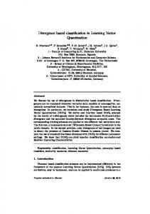
Fig. 2. Classification accuracy on building companies versus insurance agencies (top row: only cluster centers normalized to length 1, bottom row: free cluster centers with adaptable variances). The right axis shows the execution time in seconds (grey dots and lines at the bottom of each diagram).

20

100

100

Fig. 1. Classification accuracy over number of keywords on commercial banks versus soccer (top row: only cluster centers normalized to length 1, bottom row: free cluster centers with adaptable variances). The right axis shows the execution time in seconds (grey dots and lines at the bottom of each diagram).

20

60

40

100

80

fuzzy c-means

60

100

0

60

100

80

0

300

100

c-means 100

0

200

20 100

1

20

60

40

2

40

0

100

80

80 60

20 0

100

0

100

60

40

0

vector quantization

100

100

200

300

400

activation. The fuzzy learning vector quantization algorithm updated the cluster parameters once for every 100 documents.2 The results for some parameterizations of the algorithms are shown in Figures 1 (categories A vs. I), 2 (categories B vs. C), and 3 (all four major themes). The top row always shows the results for cluster centers, normalized to length 1, without variances. The bottom row shows the result for free centers with adaptable variances (diagonal covariance matrices). All results represent ten runs, which differed in the initial cluster 2 All experiments were carried out with a program written in C and compiled with gcc 3.3.3 on a Pentium 4C 2.6GHz system with 1GB of main memory running S.u.S.E. Linux 9.1. The program and its sources can be downloaded free of charge at http://fuzzy.cs.uni-magdeburg.de/˜borgelt/cluster.html.

100

200

300

400

Fig. 3. Classification accuracy on major themes (four clusters; top row: only cluster centers normalized to length 1, bottom row: free cluster centers with adaptable variances). The right axis shows the execution time in seconds (grey dots and lines at the bottom of each diagram).

0

positions and the order in which documents were processed. For the experiments with variances we restricted the maximum ratio of the variances to 1.22 : 1 = 1.44 : 1, which seemed to yield the best results over all three clustering experiments. The dotted lines show the default accuracy (obtained if all documents are assigned to the majority class). The grey horizontal lines in each block, which are also marked by diamonds to make them more easily visible, show the average classification accuracy (computed from a confusion matrix by permuting the columns so that the minimum number of errors results) in percent (left axis). The black crosses indicate the performance of single experiments. The small grey dots and lines at the top of each diagram show the performance of a

Na¨ıve Bayes Classifier trained with the corresponding subset of words. The Na¨ıve Bayes Classifier can be seen as an upper limit, while the default accuracy is a lower baseline. The bigger grey dots and lines close to the bottom show the average execution times in seconds (right axis). For all data sets the clustering process for fuzzy c-means and (fuzzified) learning vector quantization is much more stable than c-means. However, all methods seem to switch between two strong local minima for the semantically similar data sets B and C. However, the fuzzy approaches clearly seem to prefer one of them, namely the one performing better. The introduction of variances slightly improves the performance of fuzzy c-means in all cases. However, the performance for c-means is only improved for the two class problem with data sets A and I and the four class problem. The performance of fuzzy learning vector quantization is improved for the semantically more similar data sets B and C and the four class problem. However, the most remarkable observation is that fuzzy learning vector quantization needs only about 2 3 of the time needed by fuzzy clustering to obtain a result of almost equal quality. The reason is that due to the more frequent updates of the cluster parameters, fuzzy learning vector quantization converges faster, needing only about half the number of iterations in all experiments. The execution time, however, is not cut to 50%, because the more frequent updates eat up part of the gains. V. C ONCLUSIONS In this paper we transferred some ideas from fuzzy clustering, in particular the use of a covariance matrix to describe the shape and the size of a cluster, to learning vector quantization. We developed a fuzzy competitive learning scheme for these new reference vector parameters and applied our algorithm to the difficult task of clustering document collections. Our experiments showed that this approach can be used successfully for clustering collections of documents, with the learning vector quantization scheme leading to shorter execution times. In addition, it enables a truly “online” clustering, since only a fraction of the documents is needed for each update. R EFERENCES [1] R. Baeza-Yates and B. Ribeiro-Neto. Modern Information Retrieval. Addison-Wesley/Longman, Reading, MA, USA, 1999 [2] J.C. Bezdek. Pattern Recognition with Fuzzy Objective Function Algorithms. Plenum Press, New York, NY, USA 1981 [3] J.C. Bezdek, J. Keller, R. Krishnapuram, and N. Pal. Fuzzy Models and Algorithms for Pattern Recognition and Image Processing. Kluwer, Dordrecht, Netherlands 1999 [4] J. Bilmes. A Gentle Tutorial on the EM Algorithm and Its Application to Parameter Estimation for Gaussian Mixture and Hidden Markov Models. University of Berkeley, Tech. Rep. ICSI-TR-97-021, 1997 [5] H.H. Bock. Automatische Klassifikation. Vandenhoeck & Ruprecht, G¨ottingen, Germany 1974 [6] S. Deerwester, S.T. Dumais, G.W. Furnas, and T.K. Landauer. Indexing by latent semantic analysis. Journal of the American Society for Information Sciences 41:391–407. J. Wiley & Sons, New York, NY, USA 1990 [7] A.P. Dempster, N. Laird, and D. Rubin. Maximum Likelihood from Incomplete Data via the EM Algorithm. Journal of the Royal Statistical Society (Series B) 39:1–38. Blackwell, Oxford, United Kingdom 1977

[8] R.O. Duda and P.E. Hart. Pattern Classification and Scene Analysis. J. Wiley & Sons, New York, NY, USA 1973 [9] B.S. Everitt and D.J. Hand. Finite Mixture Distributions. Chapman & Hall, London, UK 1981 [10] W.B. Frakes and R. Baeza-Yates. Information Retrieval: Data Structures & Algorithms. Prentice Hall, Upper Saddle River, NJ, USA 1992 [11] I. Gath and A.B. Geva. Unsupervised Optimal Fuzzy Clustering. IEEE Trans. Pattern Analysis & Machine Intelligence 11:773–781. IEEE Press, Piscataway, NJ, USA, 1989 [12] W.R. Greiff. A Theory of Term Weighting Based on Exploratory Data Analysis. Proc. 21st Ann. Int. ACM SIGIR Conf. on Research and Development in Information Retrieval (Sydney, Australia), 17–19. ACM Press, New York, NY, USA 1998 [13] E.E. Gustafson and W.C. Kessel. Fuzzy Clustering with a Fuzzy Covariance Matrix. Proc. 18th IEEE Conference on Decision and Control (IEEE CDC, San Diego, CA), 761–766, IEEE Press, Piscataway, NJ, USA 1979 [14] F. H¨oppner, F. Klawonn, R. Kruse, and T. Runkler. Fuzzy Cluster Analysis. J. Wiley & Sons, Chichester, England 1999 [15] N.B. Karayiannis and J.C. Bezdek. An Integrated Approach to Fuzzy Learning Vector Quantization and Fuzzy c-Means Clustering. IEEE Trans. on Fuzzy Systems 5(4):622–628. IEEE Press, Piscataway, NJ, USA 1997 [16] N.B. Karayiannis and P.-I. Pai. Fuzzy Algorithms for Learning Vector Quantization. IEEE Trans. on Neural Networks 7:1196–1211. IEEE Press, Piscataway, NJ, USA 1996 [17] F. Klawonn and R. Kruse. Constructing a Fuzzy Controller from Data. Fuzzy Sets and Systems 85:177-193. North-Holland, Amsterdam, Netherlands 1997 [18] A. Klose, A. N¨urnberger, R. Kruse, G.K. Hartmann, and M. Richards. Interactive Text Retrieval Based on Document Similarities. Physics and Chemistry of the Earth, Part A: Solid Earth and Geodesy 25:649–654. Elsevier, Amsterdam, Netherlands 2000 [19] T. Kohonen. Learning Vector Quantization for Pattern Recognition. Technical Report TKK-F-A601. Helsinki University of Technology, Finland 1986 [20] T. Kohonen. Self-Organizing Maps. Springer-Verlag, Heidelberg, Germany 1995 (3rd ext. edition 2001) [21] R. Krishnapuram and J. Keller. A Possibilistic Approach to Clustering, IEEE Transactions on Fuzzy Systems, 1:98-110. IEEE Press, Piscataway, NJ, USA 1993 [22] K.E. Lochbaum and L.A. Streeter. Combining and Comparing the Effectiveness of Latent Semantic Indexing and the Ordinary Vector Space Model for Information Retrieval. Information Processing and Management 25:665–676. Elsevier, Amsterdam, Netherlands 1989 [23] M. Porter. An Algorithm for Suffix Stripping. Program: Electronic Library & Information Systems 14(3):130–137. Emerald, Bradford, United Kingdom 1980 [24] G. Salton, A. Wong, and C.S. Yang. A Vector Space Model for Automatic Indexing. Communications of the ACM 18:613–620 ACM Press, New York, NY, USA 1975 [25] G. Salton and C. Buckley. Term Weighting Approaches in Automatic Text Retrieval. Information Processing & Management 24:513–523. Elsevier, Amsterdam, Netherlands 1988 [26] G. Salton, J. Allan, and C. Buckley. Automatic Structuring and Retrieval of Large Text Files. Communications of the ACM 37:97–108. ACM Press, New York, NY, USA 1994 [27] M.P. Sinka, and D.W. Corne. A large benchmark dataset for web document clustering. A. Abraham, J. Ruiz-del-Solar, and M. K¨oppen (eds.), Soft Computing Systems: Design, Management and Applications, 881–890. IOS Press, Amsterdam, The Netherlands 2002 [28] H. Timm and R. Kruse. A Modification to Improve Possibilistic Cluster Analysis. Proc. IEEE Int. Conf. on Fuzzy Systems (FUZZ-IEEE 2002, Honolulu, Hawaii). IEEE Press, Piscataway, NJ, USA 2002 [29] H. Timm, C. Borgelt, C. D¨oring, and Rudolf Kruse. An Extension to Possibilistic Fuzzy Cluster Analysis. Fuzzy Sets and Systems 147(1):3– 16. Elsevier, Amsterdam, Netherlands 2004 [30] E.C.-K. Tsao, J.C. Bezdek, and N.R. Pal. Fuzzy Kohonen Clustering Networks. Pattern Recognition 27(5):757–764. Pergamon Press, Oxford, United Kingdom 1994 [31] I.H. Witten, A. Moffat, and T.C. Bell. Managing Gigabytes: Compressing and Indexing Documents and Images. Morgan Kaufmann, San Mateo, CA, USA 1999