Extending Noise Robust Structured Support Vector Machines to ...

Extending Noise Robust Structured Support Vector Machines to Larger Vocabulary Tasks Shi-Xiong Zhang, M. J. F. Gales Cambridge University Engineering Department Trumpington St., Cambridge, CB2 1PZ, UK {sxz20,mfjg}@eng.cam.ac.uk

Abstract—This paper describes a structured SVM framework suitable for noise-robust medium/large vocabulary speech recognition. Several theoretical and practical extensions to previous work on small vocabulary tasks are detailed. The joint feature space based on word models is extended to allow contextdependent triphone models to be used. By interpreting the structured SVM as a large margin log-linear model, illustrates that there is an implicit assumption that the prior of the discriminative parameter is a zero mean Gaussian. However, depending on the definition of likelihood feature space, a nonzero prior may be more appropriate. A general Gaussian prior is incorporated into the large margin training criterion in a form that allows the cutting plan algorithm to be directly applied. To further speed up the training process, 1-slack algorithm, caching competing hypothesis and parallelization strategies are also proposed. The performance of structured SVMs is evaluated on noise corrupted medium vocabulary speech recognition task: AURORA 4.

I. I NTRODUCTION Most automatic speech recognition (ASR) systems use generative models, in the form of hidden Markov models (HMMs) combined with class priors, the language model to yield the sentence posterior based on Bayes’ rule. Although discriminative training can be performed, the underlying models are still generative. This has led to interest in discriminative models, e.g., Structured Conditional Random Fields (SCRF) [1], and structured Log Linear Model (LLM) [2], [3], where the posterior of the word-sequence given the observation is directly modelled. For these discriminative models three important decisions need to be made: the form of the features to use; the appropriate training criterion; and how to handle continuous speech. A number of features have been investigated at the frame, model and word level [1], [4]. Features based on generative models are an attractive option as they allow state-of-the-art speaker adaptation and noise robustness approaches for generative models to be used [5]. Discriminative models are often trained using Conditional Maximum Likelihood (CML) [1], [2]. Alternatively, there has been interest in large margin [4], [6] and minimum Bayes’ risk [7] criteria. To handle continuous speech, structured discriminative models require a segmentation of the frames into word, or sub-word units. Usually these segmentations are generated by standard HMM acoustic models. Gains are observed by optimising these segmentations based on the discriminative models parameters in both training

and decoding [8]. In previous work with structured SVMs, a small vocabulary noise corrupted digit string recognition task based on whole-word HMMs was examined [4], [8]. This paper extends the previous framework of structured SVMs to handle medium/large vocabulary continuous speech recognition tasks. By interpreting the structured SVM as a large margin log-linear model, illustrates that there is an implicit assumption that the prior of the discriminative parameter is a zero mean Gaussian. However, depending on the property of log-likelihood feature space, the mean of prior should not be zeros. We relax this assumption by incorporating a more general Gaussian prior into the large margin training criterion, in a form that allows the cutting plan algorithm to be directly applied. The generalized criterion will not only lead to better trained parameters, but also help to reduces the convergence time in large scale application. In order to solve the resulted optimisation problem on larger tasks, 1-slack algorithm has to be used to replace the previous n-slack algorithm for reducing the number of constraints. To further speed up the training process, caching and parallelization strategies are also proposed. Experimental results are presented on medium to large vocabulary noise-corrupted ASR tasks: AURORA 4. II. S TRUCTURED S UPPORT V ECTOR M ACHINES n oR (r) Consider a training set with R data pairs, O(r) , wref , (r)

(r)

r=1

where O(r) = {o1 , . . . , oT } is an observation sequence and (r) (r) (r) wref = {w1 , . . . , w|w| } is the reference labels. In structured SVM for continuous speech recognition [8], our goal is to find a discriminant function αT φ(O, w; θ) that measures how well the w matches the given O, such that  ˆ = arg max αT φ(O, w; θ) w (1) w,θ

is the predicted label sequence for observations O, where α is the discriminative parameter vector, φ(O, w; θ) is a joint feature vector and θ is the hidden variable that segments the observations O1:T into |w| corresponding labels. To extend previous structured SVMs system [4], [8] to medium/large vocabulary continuous speech recognition three important decisions need to be made: at which level the hidden variable θ segments the continuous speech; the form of the features to use based on context-dependent sub-word models; and the appropriate training criterion with efficient learning algorithm.

A. Joint Feature Space This section describes the features to be used by structured SVMs for medium/large vocabulary ASR. In previous small vocabulary system [4], [8], the observations are segmented at the word level, however in order to extend the structured SVMs to medium-large vocabulary tasks data has to be segmented at sub-word level, such as phones. Given an alignment θ splits the observation sequence into |w| segments O = {Ot(w1 ,θ) , . . . , Ot(wi ,θ) , . . . , Ot(w|w| ,θ) }, where wi is the context-dependent phone label in this work. The resulting joint feature space is defined as  |w|  P δ(w ) ⊗ ϕ(O ) i t(wi ,θ)  φ(O, w; θ) ,  i=1 (2) log P (w)

where P (w) is the standard n-gram language model probability, ⊗ is the tensor product, δ(wi ) is a sparse vector indicate the position of wi in the dictionary {vk }M k=1 and ϕ(Ot(wi ,θ) ) is the generative model based log likelihood feature space for segment Ot(wi ,θ) ,     δ(w − v1 ) log(p(O; λ(v1 ) )) . .  , ϕ(O) =   (3) .. .. δ(w) =  (v ) M δ(w − vM ) log(p(O; λ )) where λ is the generative model parameters. These generative model based features allows standard noise and speaker adaptation schemes to be used to derive robust feature space. Thus the dot-product of the φ(O, w; θ) and structured SVM parameter α can be evaluated by accumulating every segment score [4] |w| P

αT φ(O, w; θ) =

T

α(wi ) ϕ(Ot(wi ,θ) )+αlm log P (w), (4)

i=1 T

T

T

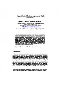
where α = [α(v1 ) , . . . α(vk ) . . . , α(vM ) , αlm ]T . Fig. 1 demonstrates an example of using Eq. (2) to construct joint feature space for data pair (O, w) given segmentation θ. +

+

…

…

“

a



b

+

c

”

…

…

…

…

… :

… … …

O

:

…

0

0

.

1

0

.

2

0

.

3

0

.

4

0

.

5

0

.

6

0

.

7

:

…

…

0

0

.

1

0

.

2

0

.

3

0

.

4

0

.

5

0

.

6

0

.

7

x W

*

y

+

z

”

:

“

x

*

y

+

z

”

“ “

“

a

*

b

+

c

a

*

b

+

c

”

”

…

…

l

o

g

( P

) w

Fig. 1. Illustration of constructing joint feature space from triphone HMMs based log-likelihood feature space.

When medium/large vocabulary ASR are considered there is an issue with above context-dependent feature space [3]. The set of context-dependent phone models {vk }M k=1 yields a very large joint feature space. Although in theory this could be used, the number of determinative model parameters becomes large. Two approaches proposed in [3] to address this problem are adopted this work. One is to reduce the dimension of the feature space ϕ(·) by selecting a small set of “suitable” generative models. Here only the generative models that share

the same observed context are included. For example, the feature space of segment Ot(a−x+c) with matched context can be expressed as   log p(Ot(a−x+c) ; λ(a−a+c) )   ..   . ϕ(Ot(a−x+c) ) =   . (5)  log p(Ot(a−x+c) ; λ(a−y+c) )  log p(Ot(a−x+c) ; λ(a−z+c) )

M1

This reduces the dimensionality of the feature space ϕ(·) from the number of context-dependent phones M to the number of mono phones M1 . The second approach is to reduce the dimension of sparse vector δ(·) by clustering the {vk }M k=1 using a phonetic decision tree. This is actually the modellevel parameter tying described in [3] where α(vi ) and α(vj ) are tied if vi and vj belongs to the same leaf node. Thus the total dimensionality of joint feature space is M2 × M1 . In this work, M1 and M2 are both set to 47, the number of mono phones. The joint feature space described above is based on a fixed segmentation. For a specific data pair (O, w), the “most likely” segmentation θˆ is considered, θˆ = arg max αT φ(O, w; θ). (6) θ

B. Large Margin Training n oR (r) Given the training data pairs, O(r) , wref , the paramer=1 ters of structured SVM can be trained by solving the following optimisation problem [8], [9]: R 1 CX 2 min ||α|| + ξr (7) α,ξ 2 R r=1 (r)

(r)

(r)

s.t. max αT φ(O(r) , wref ; θ (r) ) − max αT φ(O(r) , w∗ ; θ∗ ) θ (r)

(r)

(r)

(r)

≥ L(wref , w∗ ) − ξr ,

∀

θ∗ (r) w∗

(r)

6= wref , r = 1, . . . , R, (r)

(r)

where ξr ≥ 0 are the slack variables and L(wref , w∗ ) is (r) the loss function between reference wref and its competing (r) hypothesis w∗ . The constraints in Eq. (7) can be explained (r) as follows. For every training pair (O(r) , wref ), the best score of the correct pair should be greater than all competing pairs (r) (O(r) , w∗ ) by a margin determined by the loss. Note that (r) since the number of possible competing hypothesis w∗ is very large, there are lots of constraints in Eq. (7). Substituting the slack variable in the constraints to the objective function, the structured SVMs problem in Eq. (7) can also be expressed as a minimisation of concave

z }| R  { 1 C Xh (r) 2 T (r) (r) ||α||2 + − max α φ(O , wref ; θ ) 2 R r=1 θ (r) n oi (r) + max L(w, wref ) + αT φ(O(r) , w; θ) (8) (r)

+

w6=wref ,θ

|

{z

convex

}

where [ ]+ is the hinge-loss function. The constraints in Eq. (8) include two maximum of a set of linear functions. Each

maximum function is convex with respect to α. However, the objective function in Eq. (7), as also shown in Eq. (8), is nonconvex. To solve this non-convex optimization problem, an algorithm based on concave-convex procedure [10] and cutting plane algorithm [9] is proposed in previous work [8].

Comparison between Eq. (14) and Eq. (8) suggests that, the structured SVM used in this work can also be viewed as a large margin trained log linear model with “most discriminative” segmentation. III. G AUSSIAN P RIOR

C. Relationship with Log Linear Models The structured SVMs problems formulated in Eq. (1) and (7) can be interpreted as decoding and large margin training of log linear models. To see this, we write the posterior of the hypothesized labels w given O as a member of exponential family,   ˆ exp αT φ(O, w; θ) ˆ = , (9) P (w|O; α, θ) Z(O; α)   P where Z(O; α) = w′ exp αT φ(O, w′ ; θˆ′ ) ensures that the model is a properly normalized probability, θˆ is the best alignment that maximises posterior probability P (w|O; α, θ), θˆ = arg maxθ αT φ(O, w; θ). Recognition with this log linear model can be simply expressed as ˆ = arg max αT φ(O, w; θ) (10) ˆ = arg max P (w|O; α, θ) w w

The previous section has shown that, when training the standard structured SVMs, an implicit assumption is made that the prior distribution of α is standard Gaussian, with zero mean and identity covariance matrix. However, depending on the feature space defined in Eq. (3), the mean of prior, µ, should not be zeros. A proper mean of prior should be the one that can yield the HMM baseline performance   1 arg max µT φ(O, w; θ) = arg max log P (O|w; λ) αlm P (w) 1 w

w,θ

which implies that the value of µ is one for the correct class, zero otherwise, thus for class v1 , µ(v1 ) = [1, 0, . . . , 0]T . This motivates us to look for a more general large margin training criterion that can relax the structured SVMs prior assumption and incorporate a general Gaussian prior F˜ (α) = Flm (α) − log (P (α))

w,θ

(15)

This is equivalent to structured SVM decoding in Eq. (1). In order to train a robust model capable of generalizing well on high-dimension space even with limited data, large margin based approaches can be applied [6], [11]. If the margin for log linear models is defined as the log posterior probability (r) ratio of the reference {wref , θˆ(r) } and best competing hyˆ pothesis/alignment {w, θ}, the large margin training for log linear model can be expressed as minimising 1 XR Flm (α) = · (11) r=1 !)# " ( R (r) P (wref |O(r) ; α, θˆ(r) ) (r) max L(w, wref ) − log (r) ˆ P (w|O(r) ; α, θ) w6=w

where P (α) = N (α; µ, Σ). Thus, the objective function of structured SVMs training (Eq. (8)) can be generalized as

where [ · ]+ is the hinge-loss function. Substituting Eq. (9) into Eq. (11) and canceling out the normalization term Z(O; α), we will have R   1 Xh (r) Flm (α) = · − max αT φ(O(r) , wref ; θ (r) ) R r=1 θ (r) n oi (r) + max L(w, wref ) + αT φ(O(r) , w; θ) (12)

1 ˜ α) ˜ = ||α|| ˜ 22 + C · Flm (α ˜ + µ) F( 2

+

ref

(r)

w6=wref ,θ

+

Note that above criterion is the unregularized part of Eq. (8). To retrieve the regularization term 12 ||α||22 , a standard Gaussian distribution N (α; 0, CI) can be incorporated into the criterion as the prior probability P (α), F (α) = Flm (α) − log (N (α; 0, CI))

(13)

1 where the log prior log (N (α; 0, CI)) = − 2C αT α + const. Ignoring the terms that constant to α, yields the following regularized objective 1 F (α) = ||α||22 + C · Flm (α) (14) 2

1 T F˜ (α) = (α − µ) Σ−1 (α − µ) + Flm (α). 2

(16)

Note that the normalization term Σ−1 can always be decomposed and merged into the feature space by using trans1 ˜ formed features φ(O, w; θ) = Σ 2 φ(O, w; θ). In this work, we assume the log-likelihood features are already properly scaled, and simply using Σ = CI. In order to utilize the training framework for Eq. (8) proposed in [8], we introduce ˜ = (α − µ) to express Eq. (16) in the form of Eq. (13) α (17)

Therefore the training criterion of structured SVMs (Eq. 8) can be generalized as minimising R 1 CX ˜ 22 + ||α|| 2 R r=1

+

max

(r)

w6=wref ,θ

n

"

  (r) ˜ + µ)T φ(O(r) , wref ; θ (r) ) − max (α θ (r)

(r) L(w, wref )

T

(r)

˜ + µ) φ(O + (α

, w; θ)

o

#

(18) +

Note that once the optimal reference alignment θˆ(r) is given, then Eq. (18) can be reformulated in the form of Eq. (8) (see Algorithm 1 for more detail), where the loss is now become a score-augmented loss function (r) (r) (r) ˜ L(w, wref ) = µT ∆φ(O(r) , wref , w) + L(w, wref ) | {z } | {z } acoustic and language loss

1 acoustic

deweighting.

transcription loss

(19)

Algorithm 1: Structured SVM learning algorithm for ASR. ˜ = [0, 0, 0 . . .], µ = [1, 0, 0 . . .] ; 0. Initial: α ˜ searching the optimal reference alignment 1. Fixing α, (r) θ (r) for each training pair (O(r) , wref ) in numerator lattices using forward-backward algorithm:   (r) ˜ + µ)T φ(O(r) , wref ; θ (r) ) , ∀ r θˆ(r) = arg max (α

Algorithm 2: 1-slack Cutting plane algorithm [9] for Eq. (22). (r) Input: {(O(r) , wref ; θˆ(r) )}R r=1 , C and precision ε; Initial empty constraint set: W ← ∅; repeat /* solving the 1-slack QP using current pool */ ˜ ξ) ← arg min (α,

α,ξ≥0

1 C ˜ 22 + ξ ||α|| 2 R

θ (r)

˜T S.T. ∀ W : α

(21)

˜ by minimizing the following 2. Fixing θˆ(r) , optimise α convex upper bound using cutting plane algorithm in Algorithm 2: linear }| { R hz X 1 C (r) ˜ 22 + ˜ T φ(O(r) , wref ; θˆ(r) ) ||α|| −α (22) 2 R r=1 n oi (r) ˜ ˜ T φ(O(r) , w; θ) + max L(w, wref ) + α (r)

+

w6=wref ,θ

(r) (r) (r) ˜ where L(w, wref ) = µT ∆φ(O(r) , wref , w) + L(w, wref )

(r)

(r) , wref ; θˆ(r) ),

T

where ∆φ = φ(O , w; θ) − φ(O µ ∆φ can be viewed as an acoustic and language score loss. The ˜ can be written as decoding of structured SVMs based on α   ˆ = arg max (α ˜ + µ)T φ(O, w; θ) . w (20) w,θ

˜ One interesting property of expression (18) is that even if α is not well trained, e.g., in the earlier training stage, with a proper µ the algorithm can still generate sensible competing hypothesis and reference alignments using the max terms in Eq. (18). This is particularly helpful to reduce the convergence time in medium/large vocabulary ASR. To solve the non-convex optimisation problem with respec˜ in Eq. (18), an algorithm based on concave-convex tive to α procedure [10] is proposed in Algorithm 1. It works similar to the iteration process of EM. First, we find the “most likely” ˜ This correspond to find the segment θˆ for current parameter α. linear upper bound of the concave term of Eq. (18). Second, ˆ the resulted convex optimizawith the current segment θ, tion can be solved using 1-slack cutting plane algorithm [9] described in Algorithm 2. These two steps will go several iterations. The detail is shown in Algorithm 1. Note that the objective function in Eq. (22) is convex for α, however, solving this problem is not trivial. Because the number of constraints is exponentially large, although the number of valid constraints that actually affect the solution is limited. One existing algorithm for this type of problem is the 1-slack cutting plane algorithm summarized in Algorithm 2, where the quadratic programming (23) only has 1-slack variable. The algorithm iteratively construct a working set W of constraints. In each iteration, it computes the solution over the current W (Eq. (23)), finds the most violated constraint (Eq. (24)), and adds it to the working set. The 1-slack algorithm stops once

∆φ +

R X

r=1 r=1 (r) (r) φ(O(r) , w∗ ; θ∗ ) −

˜ ∗(r) , w(r) ) ≤ ξ L(w ref (r) φ(O(r) , wref ; θˆ(r) ).

for r = 1..R do /* Generating most competing hypothesis: */ (r)

(r)

w∗ , θ∗

n o (r) ˜ ˜ T φ(O(r) , w; θ) (24) ← arg max L(w, wref ) + α w,θ

end (r) (r) W ← W ∪ {w∗ , θ∗ }R r=1 ;

until

/* put it in the pool */

/* no constraint can be found that is violated by more than ε */

˜T α

˜ return α

3. go back to Step 1 until converge; ˜ ; 4. return α

(r)

where ∆φ =

R X

(23)

R P

r=1

∆φ +

R P (r) ˜ ∗(r) , wref L(w ) ≤ ξ+ε ;

r=1

no constraint can be found that is violated by more than the desired precision ε. IV. I MPLEMENTATION I SSUES An efficient implementation of the algorithm is important for medium to large vocabulary speech recognition. In the following we summarized several design decisions that have a substantial influence on practical efficiency. A. 1-slack optimisation There are two form of cutting plane algorithms [9], n-slack and 1-slack algorithms. An advantage of the 1-slack algorithm is the number of constraints and support vectors it produces is much smaller than n-slack case. In theory, the n-slack algorithm may add R constraints in every iteration, where R the size of training set. The 1-slack algorithm only adds a single constraint per iteration at most. In practice, for Aurora 4 experiments, 1-slack algorithms produce less then 500 active constraints at the solutions, whereas n-slack algorithms produce more than 50, 000 constraints after 20 iterations which make it impractical for medium/large vocabulary ASR. For AURORA 2 small vocabulary task, both algorithms can be applied. 1-slack algorithm only produce 24 support vectors whereas the number in n-slack case is 629. This means that in the 1-slack algorithm the QP problem (Eq. 23) on current working sets that need to be solved in each iteration are much smaller. Another interesting property about 1-slack PR algorithm (Algorithm 2) is that constraints depend on r=1 ∆φ instead of (r) (r) individual ∆φ(O(r) , wref , w∗ ). Therefore, some competing (r) hypothesis w∗ could be involved in the constraints many times. To avoid the time wasted on repeatedly searching the (r) (r) (r) same w∗ , the 10 most recently used ∆φ(O(r) , wref , w∗ ) (r) for each training observation O are cached.

2GXMK3GXMOT:XGOTOTM U

p

d

a

t

e

Z

d |

(

)

r

G

w

e

n

e

r

a

t

i

n

g

T

(

)

(

)

(

)

(

)

(

)

g

r

e

f

(

m

N

(

u

m

e

r

a

t

o

a

φ

x

x

r

r

)

­

n r

O

n

L

a

t

t

i

c

u

u

(

®

∈

m

m

e

)

n

u

r

r

)

r

i

(

O

,

w

z

;

r

e

f

)

n

m

;

m

O

°

m

a

g r

o

P

U

p

d

a

t

e

r

d

à

i

c

t

a

G

e

n

e

D

e

n

o

r

a

t

i

n

g

d

e

n

d

m m m

i

n

a

t

o

a a

d

d

e

a

t

t

i

c

e

n

∈

n

w

L

{

x x

r



e

,

(

)

T

(

,

w

r

+ φ

) )

w

f

w

w

r

e

(

,

Ú

O

r

(



;

w

) )

Ü

)

O

w

}

r

a

u

Q

u

f

:XGOTOTM6NGYK *KIUJOTM6NGYK G

e

n

e

r

a

t

i



n

g

d

e

n

O

T

a

D

e

n

o

m

i

n

a

t

d

e

o

r

g

m

a

φ

x

r

d

e

n

d

e

n

a

t

t

i

c

e

w

8

,

Fig. 2.

(

,

)

;

w

^

n



L



∈

However for 1-slack algorithm used in this work can be easily parallelized without any degradation. In theory, one could make use of up to R parallel threads, each searching the best competing hypothesis for a subset of training data. Paralleling the loop for Eq. (24) will lead to a substantial speed-up in the number of threads.

O

w

!

The diagram of training and decoding for structured SVMs.

For both the n-slack and the 1-slack algorithms, constraints that were added to the working set in earlier iterations often become inactive later. These constraints can be removed without affecting the theoretical convergence of the algorithm. This is practically useful since it leading to a relatively smaller QP to be solved in later iterations. B. Efficient search Theoretically, the large margin training criterion discussed in the previous section can be directly applied to the model training. In practice, to make the algorithms applicable to larger vocabulary ASR, there are two search sub-problems must be solved efficiently (see Fig. 2), the best reference alignment Eq. (21) in Algorithm 1 and the best competing hypothesis/alignment Eq. (24) in Algorithm 2. In previous work on small vocabulary digit string recognition task, it is feasible to search all the possible alignments and competing hypothesis in those two subproblems by using a Viterbi-style search [8]. However, it is not practical for larger tasks because the request to handle the exponential large searching space for all possible w and θ. Similar to the discriminative training in [7], numerator and denominator lattices Lnum and Lden are generated to restrict the large searching space. Then a lattice-based searching algorithm is proposed to find the best competing path (hypothesis) among the lattices. Note that αT φ(O(r) , w; θ) can be calculated arc by arc using Eq. (4) and a standard MPE approximate loss [7] can also be computed on the arc level. Thus the best competing path Eq. (24) can be efficiently achieved through an arclevel forward-backward searching over the lattice. Similarly, Eq. (21) can also be efficiently searched in the numerator lattice Lnum . For large scale applications, the computational load during training is dominated by finding the best competing hypothesis/alignment. For the n-slack algorithm, in order to run it in parallel on many machines, the sequential update mode of the standard cutting plane algorithm needs to be modified to a batch-mode update. Note that for n-slack algorithm, this parallelization will decrease the performance slightly [8]2 . 2 Because in the sequential mode n-slack algorithm, α can be updated after every training sample. This allows the algorithm to potentially find better competing w for the subsequence samples, but it can not be parallelized.

V. N OISE ROBUSTNESS In ASR, the acoustic conditions during training and testing are seldom matched. For standard generative models, modelbased compensation schemes such as Vector Taylor Series (VTS) compensation [12] are a popular and successful approach to handling this problem. When applying the same concept to structured SVMs there are two options. First, the disT T criminative model parameters, αT = [α(w˜1 ) , . . . , α(w˜M ) ], can be modified to be noise dependent. However with very limited data in the target domain, in these experiments a single utterance, this is not possible. Alternatively, the parameters λ associated with the joint feature space are modified [5]. This can be achieved using any model-based compensation scheme. In this work VTS is used. Considering just the static components of the acoustic models, the compensated mean vector and covariance matrix of component m of the generative model are given by   µ(m) = C log exp(C-1 (µ(m) + µh ) + exp(C-1 µn ) x (m)T Σ(m) = J(m) Σ(m) + (I − J(m) )Σn (I − J(m) )T x J (m)

(m)

where µx and Σx are the “clean” speech component mean vector and covariance matrix, and µn , Σn and µh are the additive and convolutional noise parameters respectively. C is the DCT matrix and J(m) is Jacobian matrix [12]. exp() and log() are element-wise exponential and logarithm respectively. The noise model parameters are estimated using maximum likelihood estimation [13]. Thus in this work structured SVM parameters are assumed to be noise-independent, whereas the generative model parameters are noise-dependent. VI. E XPERIMENTS This section describes experiments with the structured SVMs in AURORA 2 and 4. The AURORA 2 results are included to contrast the performance of 1-slack with nslack algorithms and the gains from modeling the prior. The AURORA 4 results are used to illustrate the performance of proposed structured SVMs algorithms for noise robust medium vocabulary speech recognition. AURORA 2 is a standard small vocabulary digital recognition task. The vocabulary size M is only 12 (one to nine, plus zero, oh and silence). The utterances are one to seven digits long based on the TIDIGITS database with noise artificially added. The generative models (HMMs), are 16 emitting states whole word digit models, with 3 mixtures per state. There are three test sets each includes 0 − 20dB five SNRs. Set A was used as the development set for tuning parameters for all systems, such as the penalty factor C in structured SVMs. The joint feature space is based on appended-all features in

TABLE I AURORA 2 RECOGNITION RESULTS (WER %) OF VTS BASED HMM, LOG LINEAR MODEL (LLM) [3] AND S TRUCTURED SVM S (SSVM) USING 1- SLACK , SEQUENTIAL - MODE n- SLACK ALGORITHMS AND GENERALIZED LARGE MARGIN TRAINING WITH G AUSSIAN PRIOR (A LG . 1).

Model HMM LLM (CML) SSVM (n-slack) SSVM (1-slack) SSVM (µ,1-slack)

Set A 9.8 8.1 7.6 7.6 7.5

Set B 9.1 7.7 7.2 7.3 7.1

Set C 9.5 8.3 8.0 7.9 7.9

Avg. 9.5 8.1 7.5 7.5 7.4

Eq. 3, no language model is used. The performances of VTScompensated HMM, log linear models proposed in [3] and the structured SVMs with different training algorithms and criteria are shown in Table I. Examining the results in this table, shows the benefit of using 1-slack algorithm in structured SVM where the WER are almost the same with n-slack algorithm but with much fewer support vectors (24 compared with 169) and less computation. Small but consistent gains are observed when training structured SVMs with general Gaussian prior using 1-slack algorithm (last two lines in the table). The mean of Gaussian prior is set as the α learned using 1-slack algorithm (the second last line in the table). AURORA 4 is a noise-corrupted medium to large vocabulary task based on the Wall Street Journal (WSJ) data. Our configuration repeats the previous setup where the HMM is trained from clean data (SI-84 WSJ0 part, 14 hours). The HMMs are state-clustered triphones (3140 states) with 16 components/mixture. Four iterations of VTS compensation are performed for the test data. To compare with the log linear model proposed in [3], the joint feature space of structured SVMs follows the same setup described in [3] with 47 × 47 dimensions. The log linear models and structured SVMs are trained on the multi-style data. Evaluation is performed using the standard 5000- word WSJ0 bigram model on four noisecorrupted test sets3 based on NIST Nov92 WSJ0 test set. Table II shows the AURORA4 results of structured SVMs trained using large margin criteria with a general Gaussian prior. The mean of prior is set as the parameters of CML trained log linear model. The results from last two lines shown that optimising the segmentation in the numerator lattice yields small gain in performance. Compared to the CML trained log linear models with same dimension features, proposed structured SVMs yielded a 3.4% relative reduction in WER. Note that due to too many constraints, n-slack algorithm can not be applied in AURORA 4. For this larger task, it is also impractical to train structured SVMs without considering a proper prior, since the standard large margin training with zero mean of prior convergences too slow. VII. C ONCLUSION This paper described a structured SVM framework suitable for noise-robust medium/large vocabulary speech recognition. Several theoretical and practical extensions to previous work in small vocabulary task have been made. First, the joint feature space based on word models is extended to allow contextdependent triphone models to be used. Second, by interpreting

TABLE II AURORA 4 R ECOGNITION R ESULTS . F OR SSVM, µ, MEANS LARGE ˆ MEANS MARGIN TRAINING α WITH G AUSSIAN PRIOR (A LG . 1), θ UPDATING THE SEGMENTATION IN THE NUMERATOR LATTICE .

Test Set A B HMM ML 7.1 15.3 CML 7.2 14.7 LLM MPE 7.3 14.7 LM (µ, 1-slack) 7.5 14.3 SSVM ˆ 1-slack) 7.4 14.2 LM (µ, θ, Model

Criterion

WER C 12.2 11.1 11.2 11.4 11.3

(%) D 23.1 22.8 22.7 21.9 21.9

Avg 17.8 17.4 17.4 16.9 16.8

the structured SVM as a large margin log-linear model, illustrates that there is an implicit assumption that the prior of the discriminative parameter is a zero mean Gaussian. However, depending on the definition of likelihood feature space, a non-zero prior may be more appropriate. The assumption is relaxed by incorporating a more general Gaussian prior into the large margin training criterion in a form that allows the cutting plan algorithm to be directly applied. To speed up the training process, strategies such as 1-slack algorithm, caching competing hypothesis and parallelization are proposed. The performance of structured SVMs is evaluated on AURORA 4. Gains are observed over both VTS-compensated HMM and log linear models. Kernelization of this structured SVM to support high dimensional feature spaces such as derivative feature space will be investigated in the future. ACKNOWLEDGMENT The authors would like to thank Toshiba Research Europe Ltd, Cambridge Research Lab, for partly funding this work. R EFERENCES [1] G. Zweig and P. Nguyen, “A segmental CRF approach to large vocabulary continuous speech recognition,” in ASRU, 2009. [2] M. Layton and M. Gales, “Augmented statistical models for speech recognition,” in Proc. ICASSP, Toulouse, 2006. [3] A. Ragni and M. J. F. Gales, “Structured discriminative models for noise robust continuous speech recognition,” in Proc. ICASSP, Prague, Czech Repubic, 2011. [4] S.-X. Zhang, A. Ragni, and M. J. F. Gales, “Structured log linear models for noise robust speech recognition,” Signal Processing Letters, IEEE, vol. 17, pp. 945–948, 2010. [5] M. J. F. Gales and F. Flego, “Discriminative classifiers with adaptive kernels for noise robust speech recognition,” Comput. Speech Lang., vol. 24, no. 4, pp. 648–662, 2010. [6] B. Taskar, “Learning structured prediction models: a large margin approach,” Ph.D. dissertation, CA, USA, 2005. [7] D. Povey, “Discriminative training for large vocabulary speech recognition,” Ph.D. dissertation, Cambridge University, 2004. [8] S.-X. Zhang and M. J. F. Gales, “Structured support vector machines for noise robust continuous speech recognition,” in Proc. Interspeech, Florence, Italy, 2011. [9] T. Joachims, T. Finley, and C.-N. J. Yu, “Cutting-plane training of structural SVMs,” Mach. Learn., vol. 77, no. 1, pp. 27–59, 2009. [10] A. Yuille, A. Rangarajan, and A. L. Yuille, “The concave-convex procedure (CCCP),” in Advances in Neural Information Processing Systems. MIT Press, 2002. [11] F. Sha and L. K. Saul, “Large margin hidden Markov models for automatic speech recognition,” in NIPS, 2007, pp. 1249–1256. [12] A. Acero, L. Deng, T. Kristjansson, and J. Zhang, “HMM Adaptation using Vector Taylor Series for Noisy Speech Recognition,” in Proc. ICSLP, Beijing, China, 2000. [13] H. Liao and M. Gales, “Joint uncertainty decoding for robust large vocabulary speech recognition,” Cambridge University, Tech. Rep. CUED/F-INFENG/TR552, November 2006.