EXTERNAL MEMORY TECHNIQUES FOR ISOSURFACE EXTRACTION 3 Figure 1. Typical isosurfaces are shown. The upper two are for the Blunt Fin dataset. The ones in the bottom ...
DIMACS Series in Discrete Mathematics and Theoretical Computer Science
External Memory Techniques for Isosurface Extraction in Scientific Visualization Yi-Jen Chiang and Cl´ audio T. Silva Abstract. Isosurface extraction is one of the most effective and powerful techniques for the investigation of volume datasets in scientific visualization. Previous isosurface techniques are all main-memory algorithms, often not applicable to large scientific visualization applications. In this paper we survey our recent work that gives the first external memory techniques for isosurface extraction. The first technique, I/O-filter, uses the existing I/O-optimal interval tree as the indexing data structure (where the corner structure is not implemented), together with the isosurface engine of Vtk (one of the currently best visualization packages). The second technique improves the first version of I/O-filter by replacing the I/O interval tree with the metablock tree (whose corner structure is not implemented). The third method further improves the first two, by using a two-level indexing scheme, together with a new meta-cell technique and a new I/O-optimal indexing data structure (the binary-blocked I/O interval tree) that is simpler and more space-efficient in practice (whose corner structure is not implemented). The experiments show that the first two methods perform isosurface queries faster than Vtk by a factor of two orders of magnitude for datasets larger than main memory. The third method further reduces the disk space requirement from 7.2–7.7 times the original dataset size to 1.1–1.5 times, at the cost of slightly increasing the query time; this method also exhibits a smooth trade-off between disk space and query time.
1. Introduction The field of computer graphics can be roughly classified into two subfields: surface graphics, in which objects are defined by surfaces, and volume graphics [17, 18], in which objects are given by datasets consisting of 3D sample points over their volume. In volume graphics, objects are usually modeled as fuzzy entities. This representation leads to greater freedom, and also makes it possible to visualize the interior of an object. Notice that this is almost impossible for traditional surfacegraphics objects. The ability to visualize the interior of an object is particularly 1991 Mathematics Subject Classification. 65Y25, 68U05, 68P05, 68Q25. Key words and phrases. Computer Graphics, Scientific Visualization, External Memory, Design and Analysis of Algorithms and Data Structures, Experimentation. The first author was supported in part by NSF Grant DMS-9312098 and by Sandia National Labs. The second author was partially supported by Sandia National Labs and the Dept. of Energy Mathematics, Information, and Computer Science Office, and by NSF Grant CDA-9626370. c
0000 (copyright holder)
1
2
´ YI-JEN CHIANG AND CLAUDIO T. SILVA
important in scientific visualization. For example, we might want to visualize the internal structure of a patient’s brain from a dataset collected from a computed tomography (CT) scanner, or we might want to visualize the distribution of the density of the mass of an object, and so on. Therefore volume graphics is used in virtually all scientific visualization applications. Since the dataset consists of points sampling the entire volume rather than just vertices defining the surfaces, typical volume datasets are huge. This makes volume visualization an ideal application domain for I/O techniques. Input/Output (I/O) communication between fast internal memory and slower external memory is the major bottleneck in many large-scale applications. Algorithms specifically designed to reduce the I/O bottleneck are called external-memory algorithms. In this paper, we survey our recent work that gives the first external memory techniques for one of the most important problems in volume graphics: isosurface extraction in scientific visualization. 1.1. Isosurface Extraction. Isosurface extraction represents one of the most effective and powerful techniques for the investigation of volume datasets. It has been used extensively, particularly in visualization [20, 22], simplification [14], and implicit modeling [23]. Isosurfaces also play an important role in other areas of science such as biology, medicine, chemistry, computational fluid dynamics, and so on. Its widespread use makes efficient isosurface extraction a very important problem. The problem of isosurface extraction can be stated as follows. The input dataset is a scalar volume dataset containing a list of tuples (x, F (x)), where x is a 3D sample point and F is a scalar function defined over 3D points. The scalar function F is an unknown function; we only know the sample value F (x) at each sample point x . The function F may denote temperature, density of the mass, or intensity of an electronic field, etc., depending on the applications. The input dataset also has a list of cells that are cubes or tetrahedra or of some other geometric type. Each cell is defined by its vertices, where each vertex is a 3D sample point x given in the list of tuples (x, F (x)). Given an isovalue (a scalar value) q, to extract the isosurface of q is to compute and display the isosurface C(q) = {p|F(p) = q}. Note that the isosurface point p may not be a sample point x in the input dataset: if there are two sample points with their scalar values smaller and larger than q, respectively, then the isosurface C(q) will go between these two sample points via linear interpolation. Some examples of isosurfaces (generated from our experiments) are shown in Fig. 1, where the Blunt Fin dataset shows an airflow through a flat plate with a blunt fin, and the Combustion Chamber dataset comes from a combustion simulation. Typical use of isosurface is as follows. A user may ask: “display all areas with temperature equal to 25 degrees.” After seeing that isosurface, the user may continue to ask: “display all areas with temperature equal to 10 degrees.” By repeating this process interactively, the user can study and perform detailed measurements of the properties of the datasets. Obviously, to use isosurface extraction effectively, it is crucial to achieve fast interactivity, which requires efficient computation of isosurface extraction. The computational process of isosurface extraction can be viewed as consisting of two phases (see Fig. 2). First, in the search phase, one finds all active cells of the dataset that are intersected by the isosurface. Next, in the generation phase, depending on the type of cells, one can apply an algorithm to actually generate the
EXTERNAL MEMORY TECHNIQUES FOR ISOSURFACE EXTRACTION
3
Figure 1. Typical isosurfaces are shown. The upper two are for the Blunt Fin dataset. The ones in the bottom are for the Combustion Chamber dataset. isosurface from those active cells (Marching Cubes [20] is one such algorithm for hexahedral cells). Notice that the search phase is usually the bottleneck of the entire process, since it searches the 3D dataset and produces 2D data. In fact, letting N be the total number of cells in the dataset and K the number of active cells, it is estimated that the typical value of K is O(N 2/3 ) [15]. Therefore an exhaustive scanning of all cells in the search phase is inefficient, and a lot of research efforts have thus focused on developing output-sensitive algorithms to speed up the search phase. In the rest of the paper we use N and K to denote the total number of cells in the dataset and the number of active cells, respectively, and M and B to respectively denote the numbers of cells fitting in main memory and in a disk block. Each I/O operation reads or writes one disk block.
4
´ YI-JEN CHIANG AND CLAUDIO T. SILVA
Search Phase Generation Phase marching cubes decimation Volume Data Triangles Triangles (simplification) stripping Display
Triangle Strips
Figure 2. A pipeline of the isosurface extraction process. 1.2. Overview of Main Memory Isosurface Techniques. There is a very rich literature for isosurface extraction. Here we only briefly review the results that focus on speeding up the search phase. For an excellent and thorough review, see [19]. In Marching Cubes [20], all cells in the volume dataset are searched for isosurface intersection, and thus O(N ) time is needed. Concerning the main memory issue, this technique does not require the entire dataset to fit into main memory, but ⌈N/B⌉ disk reads are necessary. Wilhems and Van Gelder [30] propose a method of using an octree to optimize isosurface extraction. This algorithm has worst-case time of O(K + K log(N/K)) (this analysis is presented by Livnat et al. [19]) for isosurface queries, once the octree has been built. Itoh and Kayamada [15] propose a method based on identifying a collection of seed cells from which isosurfaces can be propagated by performing local search. Basically, once the seed cells have been identified, they claim to have a nearly O(N 2/3 ) expected performance. (Livnat et al. [19] estimate the worst-case running time to be O(N ), with a high memory overhead.) More recently, Bajaj et al. [3] propose another contour propagation scheme, with expected performance of O(K). √ Livnat et al. [19] propose NOISE, an O( N + K)-time algorithm. Shen et al. [27, 28] also propose nearly optimal isosurface extraction methods. The first optimal isosurface extraction algorithm was given by Cignoni et al. [11], based on the following two ideas. First, for each cell, they produce an interval I = [min, max] where min and max are the minimum and maximum of the scalar values in the cell vertices. Then the active cells are exactly those cells whose intervals contain q. Searching active cells then amounts to performing the following stabbing queries: Given a set of 1D intervals, report all intervals (and the associated cells) containing the given query point q. Secondly, the stabbing queries are solved by using an internal-memory interval tree [12]. After an O(N log N )-time preprocessing, active cells can be found in optimal O(log N + K) time. All the isosurface techniques mentioned above are main-memory algorithms. Except for the inefficient exhaustive scanning method of Marching Cubes, all of them require the time and main memory space to read and keep the entire dataset in main memory, plus additional preprocessing time and main memory space to build and keep the search structure. Unfortunately, for (usually) very large volume datasets, these methods often suffer the problem of not having enough main memory, which can cause a major slow-down of the algorithms due to a large number of page faults. Another issue is that the methods need to load the dataset into main memory and build the search structure each time we start the running process. This start-up cost can be very expensive since loading a large volume dataset from disk is very time-consuming.
EXTERNAL MEMORY TECHNIQUES FOR ISOSURFACE EXTRACTION
5
1.3. Summary of External Memory Isosurface Techniques. In [8] we give I/O-filter, the first I/O-optimal technique for isosurface extraction. We follow the ideas of Cignoni et al. [11], but use the I/O-optimal interval tree of Arge and Vitter [2] as an indexing structure to solve the stabbing queries. This enables us to find the active cells in optimal O(logB N + K/B) I/O’s. We give the first implementation of the I/O interval tree (where the corner structure is not implemented, which may result in non-optimal disk space and non-optimal query I/O cost in the worst case), and also implement our method as an I/O filter for the isosurface extraction routine of Vtk [24, 25] (which is one of the currently best visualization packages). The experiments show that the isosurface queries are faster than Vtk by a factor of two orders of magnitude for datasets larger than main memory. In fact, the search phase is no longer a bottleneck, and the performance is independent of the main memory available. Also, the preprocessing is performed only once to build an indexing structure in disk, and later on there is no start-up cost for running the query process. The major drawback is the overhead in disk scratch space and the preprocessing time necessary to build the search structure, and of the disk space needed to hold the data structure. In [9], we give the second version of I/O-filter, by replacing the I/O interval tree [2] with the metablock tree of Kanellakis et al. [16]. We give the first implementation of the metablock tree (where the corner structure is not implemented to reduce the disk space; this may result in non-optimal query I/O cost in the worst case). While keeping the query time the same as in [8], the tree construction time, the disk space and the disk scratch space are all improved. In [10], at the cost of slightly increasing the query time, we greatly improve all the other cost measures. In the previous methods [8, 9], the direct vertex information is duplicated many times; in [10], we avoid such duplications by employing a two-level indexing scheme. We use a new meta-cell technique and a new I/O-optimal indexing data structure (the binary-blocked I/O interval tree) that is simpler and more space-efficient in practice (where the corner structure is not implemented, which may result in non-optimal I/O cost for the stabbing queries in the worst case). Rather than fetching only the active cells into main memory as in I/O-filter [8, 9], this method fetches the set of active meta-cells, which is a superset of all active cells. While the query time is still at least one order of magnitude faster than Vtk, the disk space is reduced from 7.2–7.7 times the original dataset size to 1.1–1.5 times, and the disk scratch space is reduced from 10–16 times to less than 2 times. Also, instead of being a single-cost indexing approach, the method exhibits a smooth trade-off between disk space and query time. 1.4. Organization of the Paper. The rest of the paper is organized as follows. In Section 2, we review the I/O-optimal data structures for stabbing queries, namely the metablock tree [16] and the I/O interval tree [2] that are used in the two versions of our I/O-filter technique, and the binary-blocked I/O-interval tree [10] that is used in our two-level indexing scheme. The preprocessing algorithms and the implementation issues, together with the dynamization of the binary-blocked I/O interval tree (which is not given in [10] and may be of independent interest; see Section 2.3.3) are also discussed. We describe the I/O-filter technique [8, 9] and summarize the experimental results of both versions in Section 3. In Section 4 we survey the two-level indexing scheme [10] together with the experimental results. Finally we conclude the paper in Section 5.
6
´ YI-JEN CHIANG AND CLAUDIO T. SILVA
2. I/O Optimal Data Structures for Stabbing Queries In this section we review the metablock tree [16], the I/O interval tree [2], and the binary-blocked I/O interval tree [10]. The metablock tree is an externalmemory version of the priority search tree [21]. The static version of the metablock tree is the first I/O-optimal data structure for static stabbing queries (where the set of intervals is fixed); its dynamic version only supports insertions of intervals and the update I/O cost is not optimal. The I/O interval tree is an external-memory version of the main-memory interval tree [12]. In addition to being I/O-optimal for the static version, the dynamic version of the I/O interval tree is the first I/Ooptimal fully dynamic data structure that also supports insertions and deletions of intervals with optimal I/O cost. Both the metablock tree and the I/O interval tree have three kinds of secondary lists and each interval is stored up to three times in practice. Motivated by the practical concern on the disk space and the simplicity of coding, the binary-blocked I/O interval tree is an alternative external-memory version of the main-memory interval tree [12] with only two kinds of secondary lists. In practice, each interval is stored twice and hence the tree is more spaceefficient and simpler to implement. We remark that the powerful dynamization techniques of [2] for dynamizing the I/O interval tree can also be applied to the binary-blocked I/O interval tree to support I/O-optimal updates (amortized rather than worst-case bounds as in the I/O interval tree — although we believe the techniques of [2] can further turn the bounds into worst-case, we did not verify the details. See Section 2.3.3). For our application of isosurface extraction, however, we only need the static version, and thus all three trees are I/O-optimal. We only describe the static version of the trees (but in addition we discuss the dynamization of the binary-blocked I/O interval tree in Section 2.3.3). We also describe the preprocessing algorithms that we used in [8, 9, 10] to build these static trees, and discuss their implementation issues. Ignoring the cell information associated with the intervals, we now use M and B to respectively denote the numbers of intervals that fit in main memory and in a disk block. Recall that N is the total number of intervals, and K is the number of intervals reported from a query. We use Bf to denote the branching factor of a tree. 2.1. Metablock Tree. 2.1.1. Data Structure. We briefly review the metablock tree data structure [16], which is an external-memory version of the priority search tree [21]. The stabbing query problem is solved in the dual space, where each interval [lef t, right] is mapped to a dual point (x, y) with x = lef t and y = right. Then the query “find intervals [x, y] with x ≤ q ≤ y” amounts to the following two-sided orthogonal range query in the dual space: report all dual points (x, y) lying in the intersection of the half planes x ≤ q and y ≥ q. Observe that all intervals [lef t, right] have lef t ≤ right, and thus all dual points lie in the half plane x ≤ y. Also, the “corner” induced by the two sides of the query is the dual point (q, q), so all query corners lie on the line x = y. The metablock tree stores dual points in the same spirit as a priority search tree, but increases the branching factor Bf from 2 to Θ(B) (so that the tree height is reduced from O(log2 N ) to O(logB N )), and also stores Bf · B points in each tree node. The main structure of a metablock tree is defined recursively as follows (see Fig. 3(a)): if there are no more than Bf · B points, then all of them are assigned to
EXTERNAL MEMORY TECHNIQUES FOR ISOSURFACE EXTRACTION
(a)
7
(b)
TS(U)
U
Figure 3. A schematic example of metablock tree: (a) the main structure; (b) the T S list. In (a), Bf = 3 and B = 2, so each node has up to 6 points assigned to it. We relax the requirement that each vertical slab have the same number of points.
the current node, which is a leaf; otherwise, the topmost Bf·B points are assigned to the current node, and the remaining points are distributed by their x-coordinates into Bf vertical slabs, each containing the same number of points. Now the Bf subtrees of the current node are just the metablock trees defined on the Bf vertical slabs. The Bf−1 slab boundaries are stored in the current node as keys for deciding which child to go during a search. Notice that each internal node has no more than Bf children, and there are Bf blocks of points assigned to it. For each node, the points assigned to it are stored twice, respectively in two lists in disk of the same size: the horizontal list, where the points are horizontally blocked and stored sorted by decreasing y-coordinates, and the vertical list, where the points are vertically blocked and stored sorted by increasing x-coordinates. We use unique dual point ID’s to break a tie. Each node has two pointers to its horizontal and vertical lists. Also, the “bottom”(i.e., the y-value of the bottommost point) of the horizontal list is stored in the node. The second piece of organization is the T S list maintained in disk for each node U (see Fig. 3(b)): the list T S(U ) has at most Bf blocks, storing the topmost Bf blocks of points from all left siblings of U (if there are fewer than Bf · B points then all of them are stored in T S(U )). The points in the T S list are horizontally blocked, stored sorted by decreasing y-coordinates. Again each node has a pointer to its T S list, and also stores the “bottom” of the T S list. The final piece of organization is the corner structure. A corner structure can store t = O(B 2 ) points in optimal O(t/B) disk blocks, so that a two-sided orthogonal range query can be answered in optimal O(k/B + 1) I/O’s, where k is the number of points reported. Assuming all t points can fit in main memory during preprocessing, a corner structure can be built in optimal O(t/B) I/O’s. We refer to [16] for more details. In a metablock tree, for each node U where a query corner can possibly lie, a corner structure is built for the (≤ Bf · B = O(B 2 )) points assigned to U (recall that Bf = Θ(B)). Since any query corner must lie on the line x = y, each of the following nodes needs a corner structure: (1) the leaves, and (2) the nodes in the rightmost root-to-leaf path, including the root (see Fig. 3(a)). It is easy to see that the entire metablock tree has height O(logBf (N/B)) = O(logB N ) and uses optimal O(N/B) blocks of disk space [16]. Also, it can be seen that the
8
´ YI-JEN CHIANG AND CLAUDIO T. SILVA
corner structures are additional structures to the metablock tree; we can save some storage space by not implementing the corner structures (at the cost of increasing the worst-case query bound; see Section 2.1.2). As we shall see in Section 2.1.3, we will slightly modify the definition of the metablock tree to ease the task of preprocessing, while keeping the bounds of tree height and tree storage space the same. 2.1.2. Query Algorithm. Now we review the query algorithm given in [16]. Given a query value q, we perform the following recursive procedure starting with meta-query (q, the root of the metablock tree). Recall that we want to report all dual points lying in x ≤ q and y ≥ q. We maintain the invariant that the current node U being visited always has its x-range containing the vertical line x = q. Procedure meta-query (query q, node U ) 1. If U contains the corner of q, i.e., the bottom of the horizontal list of U is lower than the horizontal line y = q, then use the corner structure of U to answer the query and stop. 2. Otherwise (y(bottom(U )) ≥ q), all points of U are above or on the horizontal line y = q. Report all points of U that are on or to the left of the vertical line x = q, using the vertical list of U . 3. Find the child Uc (of U ) whose x-range contains the vertical line x = q. The node Uc will be the next node to be recursively visited by meta-query. 4. Before recursively visiting Uc , take care of the left-sibling subtrees of Uc first (points in all these subtrees are on or to the left of the vertical line x = q, and thus it suffices to just check their heights): (a) If the bottom of T S(Uc) is lower than the horizontal line y = q, then report the points in T S(Uc ) that lie inside the query range. Go to step 5. (b) Else, for each left sibling W of Uc , repeatedly call procedure H-report (query q, node W ). (H-report is another recursive procedure given below.) 5. Recursively call meta-query (query q, node Uc ). H-report is another recursive procedure for which we maintain the invariant that the current node W being visited have all its points lying on or to the left of the vertical line x = q, and thus we only need to consider the condition y ≥ q. Procedure H-report (query q, node W ) 1. Use the horizontal list of W to report all points of W lying on or above the horizontal line y = q. 2. If the bottom of W is lower than the line y = q then stop. Otherwise, for each child V of W , repeatedly call H-report (query q, node V ) recursively. It can be shown that the queries are performed in optimal O(logB N + K B) I/O’s [16]. We remark that only one node in the search path would possibly use its corner structure to report its points lying in the query range since there is at most one node containing the query corner (q, q). If we do not implement the corner structure, then step 1 of Procedure meta-query can still be performed by checking the vertical list of U up to the point where the current point lies to the right of the vertical line x = q and reporting all points thus checked with y ≥ q. This might perform extra Bf I/O’s to examine the entire vertical list without reporting any point, and hence is not optimal. However, if K ≥ α · (Bf · B) for some constant
EXTERNAL MEMORY TECHNIQUES FOR ISOSURFACE EXTRACTION
9
α < 1 then this is still worst-case I/O-optimal since we need to perform Ω(Bf) I/O’s to just report the answer. 2.1.3. Preprocessing Algorithms. Now we describe a preprocessing algorithm proposed in [9] to build the metablock tree. It is based on a paradigm we call scan and distribute, inspired by the distribution sweep I/O technique [6, 13]. The algorithm relies on a slight modification of the definition of the tree. In the original definition of the metablock tree, the vertical slabs for the subtrees of the current node are defined by dividing the remaining points not assigned to the current node into Bf groups. This makes the distribution of the points into the slabs more difficult, since in order to assign the topmost Bf blocks to the current node we have to sort the points by y-values, and yet the slab boundaries (x-values) from the remaining points cannot be directly decided. There is a simple way around it: we first sort all N points by increasing x-values into a fixed set X. Now X is used to decide the slab boundaries: the root corresponds to the entire x-range of X, and each child of the root corresponds to an x-range spanned by consecutive |X|/Bf points in X, and so on. In this way, the slab boundaries of the entire metablock tree is pre-fixed, and the tree height is still O(logB N ). With this modification, it is easy to apply the scan and distribute paradigm. In the first phase, we sort all points into the set X as above and also sort all points by decreasing y-values into a set Y . Now the second phase is a recursive procedure. We assign the first Bf blocks in the set Y to the root (and build its horizontal and vertical lists), and scan the remaining points to distribute them to the vertical slabs of the root. For each vertical slab we maintain a temporary list, which keeps one block in main memory as a buffer and the remaining blocks in disk. Each time a point is distributed to a slab, we put that point into the corresponding buffer; when the buffer is full, it is written to the corresponding list in disk. When all points are scanned and distributed, each temporary list has all its points, automatically sorted by decreasing y. Now we build the T S lists for child nodes U0 , U1 , · · · numbered left to right. Starting from U1 , T S(Ui ) is computed by merging two sorted lists in decreasing y and taking the first Bf blocks, where the two lists are T S(Ui−1 ) and the temporary list for slab i − 1, both sorted in decreasing y. Note that for the initial condition T S(U0 ) = ∅. (It suffices to consider T S(Ui−1 ) to take care of all points in slabs 0, 1, · · · , i − 2 that can possibly enter T S(Ui ), since each T S list contains up to Bf blocks of points.) After this, we apply the procedure recursively to each slab. When the current slab contains no more than Bf blocks of points, the current node is a leaf and we stop. The corner structures can be built for appropriate nodes as the recursive procedure goes. It is easy to see that the entire process uses O( N B logB N ) I/O’s. Using the same technique that turns the log nearly-optimal O( N B N ) bound to optimal in building the static I/O interval B N ). (For the tree [1], we can turn this nearly-optimal bound to optimal O( N B log M B B metablock tree, this technique basically builds a Θ(M/B)-fan-out tree and converts it into a Θ(B)-fan-out tree during the tree construction; we omit the details here.) Another I/O-optimal preprocessing algorithm is described in [9]. 2.2. I/O Interval Tree. In this section we describe the I/O interval tree [2]. Since the I/O interval tree and the binary-blocked I/O interval tree [10] (see Section 2.3) are both external-memory versions of the (main memory) binary interval tree [12], we first review the binary interval tree T .
10
´ YI-JEN CHIANG AND CLAUDIO T. SILVA
Given a set of N intervals, such interval tree T is defined recursively as follows. If there is only one interval, then the current node r is a leaf containing that interval. Otherwise, r stores as a key the median value m that partitions the interval endpoints into two slabs, each having the same number of endpoints that are smaller (resp. larger) than m. The intervals that contain m are assigned to the node r. The intervals with both endpoints smaller than m are assigned to the left slab; similarly, the intervals with both endpoints larger than m are assigned to the right slab. The left and right subtrees of r are recursively defined as the interval trees on the intervals in the left and right slabs, respectively. In addition, each internal node u of T has two secondary lists: the left list, which stores the intervals assigned to u, sorted in increasing left endpoint values, and the right list, which stores the same set of intervals, sorted in decreasing right endpoint values. It is easy to see that the tree height is O(log2 N ). Also, each interval is assigned to exactly one node, and is stored either twice (when assigned to an internal node) or once (when assigned to a leaf), and thus the overall space is O(N ). To perform a query for a query point q, we apply the following recursive process starting from the root of T . For the current node u, if q lies in the left slab of u, we check the left list of u, reporting the intervals sequentially from the list until the first interval is reached whose left endpoint value is larger than q. At this point we stop checking the left list since the remaining intervals are all to the right of q and cannot contain q. We then visit the left child of u and perform the same process recursively. If q lies in the right slab of u then we check the right list in a similar way and then visit the right child of u recursively. It is easy to see that the query time is optimal O(log2 N + K). 2.2.1. Data Structure. Now we review the I/O interval tree data structure [2]. Each node of the tree is one block in disk, capable of holding Θ(B) items. The main goal is to increase the tree fan-out Bf so that the tree height is O(logB N ) rather than O(log2 N ). In addition to having left and right lists, a new kind of secondary lists, the multi lists, is introduced, to store the intervals assigned to an internal node u that completely span one or more vertical slabs associated with u. Notice that when Bf = 2 (i.e., in the binary interval tree) there are only two vertical slabs associated with u and thus no slab is completely spanned by any interval. As we shall see below, there are Θ(Bf 2 ) multi lists associated with u, requiring Θ(Bf 2 ) √ pointers from u to the secondary lists, therefore Bf is taken to be Θ( B). We describe the I/O interval tree in more details. Let E be the set of 2N endpoints of all N intervals, sorted from left to right in increasing values; E is pre-fixed and will be used to define the slab boundaries for each internal node of the tree. Let S be the set of all N intervals. The I/O interval tree on S and E is defined recursively as follows. The root u is associated with the entire range of E and with all intervals in S. If S has no more than B intervals, then u is a leaf storing all intervals of S. Otherwise u is an internal node. We evenly divide E into Bf slabs E0 , E1 , · · · , EBf−1 , each containing the same number of endpoints. The Bf − 1 slab boundaries are the first endpoints of slabs E1 , · · · , EBf−1 ; we store these slab boundaries in u as keys. Now consider each interval I in S (see Fig. 4). If I crosses one or more slab boundaries of u, then I is assigned to u and is stored in the secondary lists of u. Otherwise I completely lies inside some slab Ei and is assigned to the subset Si of S. We associate each child ui of u with the slab Ei and with the set Si of intervals. The subtree rooted at ui is recursively defined as the I/O interval tree on Ei and Si .
EXTERNAL MEMORY TECHNIQUES FOR ISOSURFACE EXTRACTION
11
u
u0
u1
u2
u3
slabs: E0 ~ E4
I4
I1
I0
u4
I5
I2 I3
I6
I7
E0
E1
E2
E3
E4
S0
S1
S2
S3
S4
multi-slabs: [1, 1] [1, 2] [1, 3] [2, 2] [2, 3] [3, 3]
Figure 4. A schematic example of the I/O interval tree for the branching factor Bf = 5. Note that this is not a complete example and some intervals are not shown. Consider only the intervals shown here and node u. The interval sets for its children are: S0 = {I0 }, and S1 = S2 = S3 = S4 = ∅. Its left lists are: lef t(0) = (I2 , I7 ), lef t(1) = (I1 , I3 ), lef t(2) = (I4 , I5 , I6 ), and lef t(3) = lef t(4) = ∅ (each list is an ordered list as shown). Its right lists are: right(0) = right(1) = ∅, right(2) = (I1 , I2 , I3 ), right(3) = (I5 , I7 ), and right(4) = (I4 , I6 ) (again each list is an ordered list as shown). Its multi lists are: multi([1, 1]) = {I2 }, multi([1, 2]) = {I7 }, multi([1, 3]) = multi([2, 2]) = multi([2, 3]) = ∅, and multi([3, 3]) = {I4 , I6 }. For each internal node u, we use three kinds of secondary lists for storing the intervals assigned to u: the left, right and multi lists, described as follows. For each of the Bf slabs associated with u, there is a left list and a right list; the left list stores all intervals belonging to u whose left endpoints lie in that slab, sorted in increasing left endpoint values. The right list is symmetric, storing all intervals belonging to u whose right endpoints lie in that slab, sorted in decreasing right endpoint values (see Fig. 4). Now we describe the third kind of secondary lists, the multi lists. There are (Bf − 1)(Bf − 2)/2 multi lists for u, each corresponding to a multi-slab of u. A multi-slab [i, j], 0 ≤ i ≤ j ≤ Bf − 1, is defined to be the union of slabs Ei , · · · , Ej . The multi list for the multi-slab [i, j] stores all intervals of u that completely span Ei ∪ · · · ∪ Ej , i.e., all intervals of u whose left endpoints lie in Ei−1 and whose right endpoints lie in Ej+1 . Since the multi lists [0, k] for any k and the multi lists [ℓ, Bf−1] for any ℓ are always empty by the definition, we only care about multi-slabs [1, 1], · · · , [1, Bf−2], [2, 2], · · · , [2, Bf−2], · · · , [i, i], · · · , [i, Bf−2], · · · , [Bf−2, Bf−2]. Thus there are (Bf − 1)(Bf − 2)/2 such multi-slabs and the associated multi lists (see Fig. 4). For each left, right, or multi list, we store the entire list in consecutive blocks in disk, and in the node u (occupying one disk block) we store a pointer to the starting position of the list in disk. Since in u there are O(Bf 2 ) = O(B) such pointers, they can all fit into one disk block, as desired.
12
´ YI-JEN CHIANG AND CLAUDIO T. SILVA
It is easy to see that the tree height is O(logBf (N/B)) = O(logB N ). Also, each interval I belongs to exactly one node, and is stored at most three times. If I belongs to a leaf node, then it is stored only once; if it belongs to an internal node, then it is stored once in some left list, once in some right list, and possibly one more time in some multi list. Therefore we need roughly O(N/B) disk blocks to store the entire data structure. Theoretically, however, we may need more disk blocks. The problem is because of the multi lists. In the worst case, a multi list may have only very few (