fect transistor (FET) devices. ... modeling FETs is the use of an equivalent circuit. The ..... [9] W. Curtice, âA MESFET model for use in the design of GaAs inte-.
Extraction and Modeling Methods for FET Devices R. Follmann, J. Borkes, P. Waldow, and I. Wolff
T
here are many ways of modeling field effect transistor (FET) devices. Physics-based models do not require any kind of measurements. They are completely based on the physics of the FET and simulate its behavior solving semiconductor equations for different geometries and doping profiles. Although these models are very flexible, they are have not been useful to circuit design engineers because of their huge amount of computing time. The most common way in modeling FETs is the use of an equivalent circuit. The elements of the circuit are extracted using different kinds of measurements and afterwards described using either mathematical equations or look up tables. Both, equations and tables must allow interpolation between non-measured DC values. This article describes an efficient method for FET modeling that requires a minimum number of measurements, namely only a set of small signal scattering parameters at different bias points. The proposed method is based on spline functions, takes into account thermal and noise effects, allows a scaling of different FET device geometries, and is available in commercial CAD software like Agilents Series IV or ADS.
Equivalent Circuits The equivalent circuit of a FET can be divided into two parts: constant and bias independent extrinsic elements and a bias dependent intrinsic part. Each element has a physical meaning. The extrinsic elements, for example, describe pad capacitances or resistivity of the transistor lines whereby the intrinsic charge zone of the FET is represented by the gate-source and gate-drain capacitances (Figure 1). We propose an equivalent circuit [1] based on the well known 15 element circuitry [2,3]. Some changes (Figure 1), however, are required for the nonlinear modeling: ● All intrinsic elements are extracted bias dependent (both voltages) ● The current source IDS is replaced by measured IV-curves IDS(VGS, VDS) September 2000
Two Schottky diodes, which can be determined from the measured scattering parameters, describe its compression behavior ● The intrinsic conductance g is calculated by optimizing small signal scattering parameters at each bias point. All intrinsic elements depend on two bias voltages VGS and VDS . The determination procedure of the extrinsic elements is well known. Using so called cold-scattering parameter measurements with VDS = 0 V, VGS < VP , and VGS >> 0 V, whereby VP is the pinch-off voltage of the device, R S can for example be calculated as ●
R S = Re{z 12 ( f )}.
(1)
The extraction of the extrinsic elements should not depend on the frequency f. In most cases, the extrinsic elements can also be determined through an optimization process comparing measured and simulated scattering parameters. In that case, varying intrinsic elements with varying extrinsic ones must be taken into account. The determination of the intrinsic elements is a bit more complicated, as can be seen in the equation for the extraction of the intrinsic capacitance
c GS (VGS ,VDS ) =
f2
∑
f = f1
{ {
} }
1 Im y 11 (VGS ,VDS ) ω + Im y (V ,V ) GS DS 12
(
)
/ n f 2 − n f1 .
(2)
Here, the median over a frequency range ( f 1 K f 2 ) for n measured frequency points must be calculated. Figure 2 shows a typical example of the intrinsic gate-source capacitance in dependence of both VGS and VDS. Many FET models show two main problems: ● dc simulation and intrinsic output conductance GDS cannot be fit simultaneously for high frequencies [4] ● Determining a charge of a capacitance, which depends on two bias voltages, by a partial integration introduces new elements (transcapacitances) to the small signal equivalent circuit [4,5], to pre-
ISSN 1527-3342/00/$10.00©2000 IEEE
1
serve the consistence between small and large signal equivalent circuit. The first problem can be solved using a topology shown in Figure 1, blocking capacitor C in series with bias dependent new output conductance g(VGS ,VDS )). A general solution for the second problem is given as follows.
Large Signal Modeling For harmonic balance simulation purposes, the charge of each nonlinear capacitance must be calculated: V1
Q1 ( v 1 ) = ∫ C( ~v 1 ) d~v 1 . 0
(3)
However the charge of a capacitance depending on two voltages is a function of the integration path v1
Q2 ( v 1 , v 2 ) = ∫ C( ~v 1 , v 2 ) d~v 1 + Q1 ( v 2 ). 0
(4)
Therefore, a significant discrepancy between small and large signal models for low input power can often be noticed. For low input power, the large signal model must turn into the small signal model [4]. One way to solve this problem is to develop the voltage-dependent capacitance into a series n
C(V1 ,V2 ) = ∑ c i (V1 ) ⋅ Ti (V2 ), i=0
(5)
where c i (V1 ) and Ti (V2 ) can be integrated separately. This results in many additional steps of calculation and further inaccuracy. An easier way to integrate a capacitance depending on two bias voltages into a large signal circuit simulator is to transform a charge source into its equivalent current source. The whole charge QG under the FET gate can be divided into two parts: a gate-source part QGS and a gate-drain part QGD . The large signal current of the gate-source part of the charge, for example, can then be calculated using (4): iGS =
∂QGS ( v GS , v DS ) ∂v = C′ GS ( v GS , v DS ) ⋅ GS . ∂t ∂t
(6)
Since there is no dc current through a capacitance, C’ is called a parametric capacitance. For the capacitance C’GS, usually a Taylor approximation of the small signal capacitance c GS is used.
Integration into CAD Software In (6), the time derivative of a voltage dv/dt is needed, although most nonlinear frequency domain simulators do not give any access to these voltages or to any internal time step they use. 2
The time derivative of any voltage in a nonlinear frequency domain circuit simulation software (like HP-EEsofs series IV/ADS) can be calculated using the trick shown in Figure 3. Into the nonlinear node (Figure 3) flows a charge equal to q = Cv. The voltage v is that voltage, of which the time derivative is needed. During the harmonic balance analysis, the simulator calculates the current iR through the resistor R as iR = q& = C ⋅ v&.
(7)
The voltage across the terminal of the resistor and therefore the potential at the node, where the charge flows in, can be calculated as v R = iRR = CR ⋅ v&.
(8)
Many experiments with the harmonic balance engine of HP-EEsofs series IV/ADS have shown that values of R = 100 Ω and C = 1e-16 F are well suited for any harmonic balance calculation case. In order to simulate even dispersion effects, a value for C can be set in the µF area. In our model, one of these constructions is used for every nonlinear capacitance (Figure 1). To check, whether that implementation into a harmonic balance simulator is correct or not, small signal simulation of scattering parameters must be compared to scattering parameters that have been calculated using a large signal test bench with very low (-30 dBm) input power. In Figure 4, this verification can be seen for an N = 4 finger Wt = 50 µm HEMT for the scattering parameter s21 . For very low input power, both the small signal and the large signal case result in identical scattering parameter simulation. For higher input power (0 dBm), the compression behavior of the device can be seen in the large signal simulation case. All other scattering parameters must show the same agreement, if the implementation is consistent. The values of the intrinsic elements (see Figure 1, for c GS example) should be described either as mathematical functions or using spline functions. The advantage of spline functions is that no equation coefficients have to be calculated, whereby as a drawback measurements have to be very accurate. Both mathematical description and spline functions must take care for a smooth extrapolation outside the measured region for harmonic balance calculation purposes. This is also true for any exponential function. These functions should be linearized for large arguments. For many CAD software packages, the element descriptions must be transformed to the intrinsic transistor voltages. Neglecting the gate current this can be done using (9): Vgs′ = Vgs − I ds (Vgs ,Vds ) ⋅ R S Vds′ = Vds − I ds (Vgs ,Vds ) ⋅ ( R D + R S ).
(9) September 2000
S( N ref ) = S(Wt ,ref ) = 1.
Diode Currents Gate-source and gate-drain diode (Figure 1) can be extracted using different methods. One method is to dc-measure both diode currents in parallel and solve both diode equations iteratively. Another method is to use the measured IV output characteristic at VDS = 0 V in order to get the diode current I G in dependence of VGS . In order to save extensive dc measurements and computing time in solving diode equations, even small signal scattering parameters can be used for calculation of diode saturation current IS and ideality factor n:
{ } = ∂∂UI
−Re y 12
D
=
GD
U IS exp GD . nVt nVt
(10)
Scaling, Temperature, and Noise In most approaches, simple scaling functions are proposed in terms of doubling the transistor size is equivalent to double the output current and the intrinsic capacitances and halving the resistances. Our approach [6,7] measures and extracts the devices out of a matrix of transistors with varying numbers of gate fingers and different gate finger widths. From the scaling calculation, we take a cross of devices consisting of one line with constant number N of gate fingers and another line of constant gate finger width Wt . The intersection point of the two lines represents the reference device. Scaling the extrinsic elements is a simple procedure. Only the relationship between two bias independent elements has to be taken into account. But all intrinsic elements of a FET device depend on two voltages. Therefore, the usually used equation device area of new device device area of reference device
(11)
is not as accurate as our proposed equation (12) for calculating scaling coefficients c for the intrinsic elements
c new =
∑
V GS , V DS
Eref (VGS ,VDS ) Escal (VGS ,VDS ) nV GS ,V DS
SI ( x ) = a Ix ⋅ x + bIx ,
(14)
where x stands for either N or Wt . The overall scaling function for the intrinsic elements can be superposed (15)
These functions can simply be expanded and are therefore suitable for any kind of simulation software and any kind of nonlinear model. The proposed theory can also be used for calculating temperature dependence of FET devices. Thus, nonintrinsic element grids for devices with different chip sizes are scaled, but dc output characteristics of the same device at different temperatures. Neglecting the temperature dependence of the capacitances [8], the temperature dependence of a FET can be expressed taking into account only dc characteristics at different temperatures and temperature variation of the resistances. With rising temperature, the IDS current drops. For very high and very low temperatures, saturation effects can be seen. In a first approach, the temperature behavior of the output characteristics is simulated using (16) a 1 T ⋅ T + b1 T S1 IDS ( T ) = a 2 T ⋅ T + b2 T a ⋅ T + b 3T 3T
for T < T1 for T1 ≤ T < T2 for T ≥ T2
R i ( T ) = R i ( T0 ) ⋅ [ γ Ri ( T − T0 ) + 1]
(16)
where T1 and T2 limit the median temperature range from saturation effects of very low and very high temperatures. For noise calculation, adapted noise equations [8] are used. For a conductance of a noise resistance (17) gR =
ith2 4kT0∆f
⋅
Tsim T0
(17)
is used. The channel noise is modeled using (18)
. (12)
In (12), Eref is the reference grid for the reference device, Escal is the grid of the device, to that the reference device should be scaled and n is the number of bias points taken into account for the calculation of the scaling coefficients. The scaling coefficient for the reference device is scaling with N as well as scaling with Wt September 2000
In a first approximation, all scaling coefficients are interpolated using linear functions, whereby a is the slope and b the y-axis interception point of the straight line
SI ( N ,W ) = SI ( N ) ⋅ SI (W ).
It can be shown that the error using scattering parameters for calculating diode currents is much less than the one using dc values and solving an equation system iteratively. Equation (10) can simply be solved using the method of linear regression.
c old =
(13)
a 1 I f 2 T0 ∂ I ds Tsim ⋅ , g Ids = k f dsb + f 3 Tsim ∂ Vgs T0 4kT0
(18)
where Tsim is the temperature for which the noise parameter should be calculated, T0 is the actual temperature, k f and a f are noise coefficients, and b is the frequency exponent. 3
Verifications The model has been verified on various MESFETs and HEMTs and was found to work very well within complex circuits containing more than one FET. In the meantime, a very complex Tx/Rx module has been successfully realized just using one scaleable transistor simulation file following the proposed approach. To demonstrate the models applicability to a four-finger 50 µm gate width HEMT (T420), the simulations of dc curves, small signal S-parameters, and a frequency-times-five multiplier are compared to measurements. In addition, an error grid containing the frequency-average complex difference between small signal S-parameter measurement and simulation for each bias point is given. Figure 5 shows the IV-curves simulation in a perfect agreement to the measurement. As shown in the S-parameter error grid (Figure 6), the simulation of small signal S-parameters is in very good agreement to the measurement even for a large range of bias points, so that the reader will get a feeling of the small signal models quality from the total error grid. The average error is less then 5%. For very high positive voltages of Vgs, the error increases due to measurement and spline interpolating inaccuracies. But in comparison to the Curtice cubic model [9], the linear simulation still is very good. In Figure 7, an up-scaling to an N = 8 finger Wt = 75µm device of the same technology is shown in comparison to the measurement at a bias point of VGS = 0 V and VDS = 2V. Figure 8 shows a down-scaling of the same device, this time at a bias point of VGS = 0V and VDS = 0V. Both simulations are in very good agreement to measurement, although the up-scaled device has twice the number of gate fingers and 1.5 times the gate finger width of the reference device. Similar good results can be achieved for any other bias condition. For testing the quality of the whole model, even for generating harmonics, a frequency-times-five multiplier (Figure 9) was simulated and measured. This extremely nonlinear circuit converts an input signal of 5 GHz to an output signal of 25 GHz using the 5th harmonic of the first transistor stage, which is driven into compression. The second stage serves as a buffer amplifier. In Figure 10, the measurement of the 5th harmonic can be seen together with the simulation of the circuit using a Curtice cubic model [9] and the TOPAS [1, 6, 7] model using the calculation theory described previously. As can be seen, the simulation using the
4
TOPAS model is in good agreement to measurement, whereby the Curtice model has some seriously convergence problems in the power range between -5 and +5 dBm input power. Even simulation results are better using our approach. All other harmonics show similar excellent results.
Advantages A state of the art method of nonlinear transistor modeling has been described using a minimum number of measurements. The proposed method has several advantages compared to other models: ● Small and large signal simulation results are identical for low input power ● Very good agreement between simulation and measurement for small signal, large signal and static simulation ● Valid for all bias points ● Scaling, temperature, and noise included ● Complete extraction and simulation within a very short time (