extraction of hydrographic networks from satellite images ... - CiteSeerX
Recommend Documents
Sensing Images Using an Oscillator Network with Weight. Adaptation. Xiuwen Liu, Ke Chen, and DeLiang Wang. AbstractâWe propose a framework for object ...
Keywords: remote sensing, Fruška gora, CORONA satellite images, automated digital surface model extraction. INTRODUCTION. By 2002 the Department of ...
images from the CORONA program in monitoring surficial mass movement ... Thus it was neces- sary to review processing methods available for the CO- ..... www.ipi.uni-hannover.de/fileadmin/institut/pdf/schenk.pdf. Timár G. â Molnár G.
The accuracy assessment of the obtained vectorized road network proved the ability of the proposed method in sub-pixel road extraction. * Corresponding ...
Paris, Shanghai, and Khartoum. ... Convolution Neural Network (CNN) for high resolution satellite image ... segmentation boundaries in high resolution satellite.
Email: [email protected]. KEYWORDS: Feature Extraction, MATLAB, ANN, Land use, Land cover. ABSTRACT: Feature extraction is the most important ...
Aug 4, 2016 - registration [3], transportation applications [4,5], personal navigation .... VHR images, say at 1 m ground resolution, cars, trees that occlude ..... of the plate and ball voting fields as the most time consuming parts of ..... The res
Grid system for flood extent extraction from satellite images. Authors; Authors and affiliations. Nataliia Kussul; Andrii Shelestov; Serhiy SkakunEmail author.
Dec 12, 2016 - To cite this article: Mehdi Maboudi, Jalal Amini, Michael Hahn & Mehdi Saati (2017) Object- based road extraction from satellite images using ...
... sensed image can be divided into five categories; trees, roads, buildings, sandy ..... (Audet, Charles , & Dennis, 2003) providing theoretical background on the ...
Ehab Salahat, Hani Saleh, Andrzej S. Sluzek, Baker Mohammad, Mahmoud Al-Qutayri, and ... Street extraction is a challenging task due to the associated.
their discriminatory ability in correct classifying images as either belong- ing to contractions or ... an efficient feature extraction methodology based on anisotropic image process- ..... diagno-sis using online learning and differential evolution.
face extraction problem from noisy volumetric images. This is since they ...... Available online http://www.cs.tut.fi/ jupeto/dmnoisy.pdf. [13] D.J. Williams and M.
In this paper we present an approach to the automatic extraction of roads from aerial images. We argue that a model for road extraction is needed in every step ...
ing sub-areas of Machine Learning: deep networks [Lee et al., 2009b], [Lee et al., ... proach is inspired by and extends the idea of penalty logic. [Pinkas, 1995] ...
Inc. Texas, Houston. http://www.derive.com 2002. [18] R. Setiono, âGenerating ... University of Sheffield, UK. [21] http://www.auknomi.com/webFiles/wisconsin-.
paper, we first give a short review of these methods proposed for text detection and recognition in web images; then a framework to extract from web images is ...
We propose to tackle the problem using a model based on marked point ... MPP framework has been defined on the space of arbitrarily-shaped objects allowing more accurate extraction ..... Then, a level set segmentation is performed in order to refine
... viewpoint Pv. Then the intensity Ii is calculated by the following equation[25]. .... computation for generating images takes a long time. Therefore, the number of ...
Technical University of Athens, Greece - [email protected], [email protected] ... The study area was located in the Death Valley, Nevada, USA.
necessary) to develop methods at object level rather ... between the objects are perceivable and exploitable. ... The vertex attributes are .... The mask center is.
Abstract. A technique for extracting intrinsic images, including the reflectance and illumination images, from a single color image is presented. The technique first ...
Robust Extraction of Text from Camera Images. S P Chowdhury. S Dhar. A K Das. B Chanda. K McMenemy. Intelligent Systems & Control. S/W Engineer.
Jul 16, 2000 - urban/suburban databases, such as road network, building reconstruction, 3D city modeling and other GIS related applications. For.
extraction of hydrographic networks from satellite images ... - CiteSeerX
Caroline Lacoste â, Xavier Descombes â, Josiane Zerubia â and Nicolas Baghdadi +. â Ariana, joint research group CNRS/INRIA/UNSA. INRIA, 2004 route ...
EXTRACTION OF HYDROGRAPHIC NETWORKS FROM SATELLITE IMAGES USING A HIERARCHICAL MODEL WITHIN A STOCHASTIC GEOMETRY FRAMEWORK. Caroline Lacoste ∗ , Xavier Descombes ∗ , Josiane Zerubia ∗ and Nicolas Baghdadi + ∗
Ariana, joint research group CNRS/INRIA/UNSA INRIA, 2004 route des Lucioles - BP 93 06902 Sophia Antipolis cedex - FRANCE Email: [email protected] Web: http://www-sop.inria.fr/ariana/
ABSTRACT This article presents a two-step algorithm performing an unsupervised extraction of hydrographic networks from satellite images, within a stochastic geometry framework. First, the thick branches of the network are detected by a segmentation algorithm based on a Markov random field. Second, the line branches of the network are extracted using a recursive algorithm based on a hierarchical model of hydrographic network, in which the tributaries of a given river are modeled by an object process in the neighborhood of this river. Optimization of the object process is done via simulated annealing using a reversible jump Markov chain Monte Carlo algorithm. We show experimental results on a satellite radar image. 1. INTRODUCTION Image analysis is an important tool for cartographers to optimize the time spent on ground while improving the accuracy of the final document. With the availability of remotely sensed images and advances in computing technologies, many methods have been developed in order to extract cartographic items for updating geographical data. In this context, we have been interested in extracting hydrographic networks constituted of rivers and their tributaries from remotely sensed images. For remote sensing applications, classification is one of the most commonly used techniques to extract quantitative information from images. Markov Random Fields (MRFs), known for their robustness with respect to noise, allows to introduce explicitly a prior knowledge on the spatial structure of the analyzed images through local conditional probabilities [1]. Nevertheless, it remains difficult to incorporate strong geometrical constraints in such models, since MRFs are defined locally. In order to exploit the geometrical and topological characteristics of the hydrographic networks, we use object processes, that are random sets of objects whose number of objects is a random finite variable. Such models, introduced in image processing in [2], provide the same type of stochastic properties as those of MRFs, while incorporating strong geometric constraints. Interactions between objects are taken into account in the density of the process, which allows to incorporate constraints on the network topology. In [3, 4], unsupervised road network extraction is performed using object processes whose objects are interacting line segments. These The first three authors thank the BRGM for partial funding and for providing radar data.
BRGM, French Geological Survey 3, avenue Claude-Guillemin - BP 6009 45060 Orléans - FRANCE Email: [email protected] Web: http://www.brgm.fr/ +
models lead to continuous extracted line networks with few omissions and overdetections. This modeling is extended in [5] to more complex objects: the objects are interacting polylines composed by an unknown number of segments, which improve the accuracy of the detection. At the end of the algorithm, each detected polyline corresponds to the central axis of a road or a river of constant width. In this paper, we use the same type of modeling as in [5] while exploiting the fact that the hydrographic network has a tree structure. As the manipulation of complex objects is computationaly expensive, we propose to initialize the algorithm by an extraction of the thick branches using a MRF. Then, the line branches of the network are extracted using a recursive algorithm based on a hierarchical model of hydrographic networks, in which the tributaries of a detected river are modeled by a polyline process in the neighborhood of this river. 2. DATA The data used in this study are a radar image (ERS) over a region of French Guyana provided by the BRGM (French Geological Survey). This image is shown in Figure 1. The sought-after cartographic item is the hydrographic network. The latter is characterized by a tree structure, where the main river is the root of the tree and its tributaries are branches from which other branches can be generated. The radar imagery is well-adapted, as rivers correspond to dark regions in the image in a light background. The main difficulty is to extract the fine branches (width lower than 3 pixels) whose detection is perturbed by speckle noise (radar). 3. FIRST SEGMENTATION To extract the rivers from radar images, we first propose a segmentation method based on a Markov random field. We suppose that there are two labels: cR corresponding to the rivers and cB corresponding to the background. Given the data field Y , our goal is to find the label field X. Embedded in a Bayesian framework, a natural candidate for X is the Maximum A Posteriori (MAP) estimator: XˆMAP = argmax P(X|Y ) = argmin U(X|Y ) X
X
(1)
where the energy U can be written as follows: U(X|Y ) = U1 (X) +U2(Y |X) where U1 is the prior term and U2 the data term.
(2)
c Figure 1: Radar image (ERS) of French Guyana of size 1098x884 and resolution 12.5 meter BRGM.
To regularize the classification while preserving the edges we define a boolean line process as proposed by [6] for image restoration. This process explicitly represents the presence of an edge in the image. The prior term is then given by: U1 (X) = b
dxs 6=xt (1 − b)
(3)
where b is a positive weigh, < s,t > denotes the pair of neighboring pixels s and t, xs is the value of X at pixel s, b denotes the value of the line field B between the pixels s and t, and dA is equal to 1 if A is true and 0 if not. In order to be efficient, we consider the process line as known. We use a “Canny-Deriche” filter to compute the line field [7]. The data term is then defined as follows: U2 (Y |X) =
where g(.|m, s ) is the Gaussian log-likelihood function of mean m and standard deviation s , mR and sR (resp. mB and sB ) correspond to the empirical mean and variance of the pixels whose label is cR (resp. cB ). The values mR , sR , mB and sB are updated during the optimization algorithm at each scanning of the image. Instead of estimating the MAP with a simulated annealing, we use the Iterated Conditional Mode algorithm which converges to a local minimum of the energy [8]. This simple method gives good results in a few seconds (with a processor 1 GHz). All the thick branches (larger than 3 pixels) are detected and the few false alarms can be easily removed by a morphological post-processing as shown in Figure 2. Nevertheless, the line branches (lower than 3 pixels) are not detected. Some tests have been performed using more elaborate models and simulated annealing but, despite some improvements, a large part of the lines of the network was still omitted.
Figure 2: Segmentation using a MRF and a morphological post-processing.
4. NETWORK MODELING USING STOCHASTIC GEOMETRY 4.1 Hierarchical modeling In this section, we model the network by a collection of objects having a hierarchical structure, each object corresponding to a river. The first level of the hierarchy represents the main rivers of the observed scene. For each object of the first level - considered as known - a process is defined in its neighborhood to model the tributaries of the corresponding main river. For each tributary, a process is defined in its neighborhood to model its tributaries. And so on.
4.2 Process defined in the neighborhood of an object Let C be the set of detected objects. Each object c ∈ C is described by a polyline corresponding to its central axis and its projection in the image S(c). Let EC be the equivalent in continuous of S(c). EC is thus defined as a bounded set of R2 which is delimited by the edges of the object c. For each object c ∈ C, we defined a reference object process within the influence zone V (c) ⊂ R2 of c, defined as follows: d(p, c) < dmax p∈ / EC p ∈ V (c) ⇔ (5) c = argmin d(p, c) C
where d(p, c) denotes the distance between p and the edges of c. The figure 3 illustrates this definition. Each object of the
reference process is a polyline described by its initial point p ∈ V (c), and an unknown number n of segments, which are described by their length and their orientation. Under the reference process law, the number N of polylines follows a Poisson law, the initial points are uniformly distributed in V (c) and the other parameters are independently and uniformly distributed in their respective state space. To introduce an a priori on polyline shapes and interactions between polylines, we then specify the process by a prior density h p with respect to the reference process law. The expression of h p is the following: U1 (x))
(6)
x∈Xc
where Xc is the configuration of objects defined with respect to c and U1 is given by: |S(s)| +¥ if ∃s ∈ Xc : |S(s) ∩ S(C ∪ Xc \ s)| > 2 n−1 U1 (x) = U12 (a j , a j+1 ) if not U11 (n) + j=0
g(v|mR , sR ) > g(v|mB , sB )
(7) The prior term U1 forbids the overlapping of more than 50% of the area S(s) covered by a segment s of a polyline with the area of the rest of the network. Moreover, it favors long polyline through a potential U11 on the number of segments n composing a polyline x. It favors slight curvature through a potential U12 on pairs of successive orientations {a j , a j+1 }. For more details, see [9]. The incorporation of data properties is done by a data term hd based on a local contrast measure of the projection of
(8)
where g(.|m, s ) is the Gaussian log-likelihood function, mR and sR (resp. mB and sB ) correspond to the empirical mean and variance of the rivers (resp. background) detected using a MRF. The other pixels of the mask are assigned to B. The line width (supposed to be lower or equal than 3 pixels) is thus implicitly taken into account through observations. The contrast between S and B is evaluated using the statistical measure usually used to perform Student t-test, which allows to evaluate if the means of two sets are significantly different. Let M(Xc ) be the set of pixels belonging to the masks of the segments of the configuration Xc . Each pixel p ∈ M(Xc ) belongs to at least one mask. For each mask M that includes p, we have computed a contrast value vM . The local contrast value at pixel p is then the minimal contrast value computed on these masks: vc (p) = min vM (p) . Finally, the data term M/p∈M
is given by:
Figure 3: Influence zones.
h p (Xc ) = exp(−
the current configuration S(Xc ) in the image with its nearby background. To compute the contrast value, we associate to each segment s composing the polylines a mask of pixels Ms = (S, B) composed of: • an internal region S corresponding to the object in the image; • an external region B corresponding to the nearby background. S is composed of the discrete segment and the neighboring pixels in the normal direction with value v satisfying:
hd (Xc ) = exp(−
uc (p)
(9)
p∈M(Xc )
where uc (p) is a potential directly based on the local contrast measure vc (p). The complete density of the process is then given by: h(Xc )
h p (Xc ) hd (Xc )
(10)
5. NETWORK EXTRACTION USING A HIERARCHICAL MODELING 5.1 Initialization The network initialization is based on the segmentation using a MRF presented in section 3. The morphological postprocessing provides a connex component for each network composed of a main river, its tributaries, the tributaries of these tributaries, etc. To go from pixels to objects, we propose a two step algorithm which consists of: first, the extraction of the skeleton of each connex component; second, the polygonalization of this skeleton in order to obtain a tree of polylines, each polyline corresponding to the central axis of a river. This first step provides thus a tree of objects corresponding to the surface part of the network. We have then a partial representation of the detected objects: the ends of branches are omitted as the river width decreases in direction of the spring. To extend each polyline c, we propose to estimate the set of the final parameters vˆ (orientations and lengths of final segments) which minimizes the energy associated to the extended polyline cv = (c, v): vb = argmin[U1 (cv ) + v
uc (p)] p∈M(cv )
(11)
The optimization is done via a simulated annealing using a Monte Carlo Markov Chain (MCMC) algorithm. The MCMC algorithm - which consists in simulating a discrete Markov Chain which converges toward the measure of interest - is the Metropolis-Hastings algorithm [10]. At each step, a transition from the current state to a new state is proposed according to a proposition kernel which is composed of several sub-kernels, each corresponding to a reversible move. The transition is accepted with a probability given by a ratio which is computed so that the detailed balance condition is verified (condition under which the generated Markov chain converges toward the process measure). The perturbations proposed in the sampling algorithm do not modify the initial parameters of the considered polyline. We use two reversible moves: “add-and-remove” a segment to the end of the polyline; “translation” of a point of the polyline. 5.2 Generating new branches The hierarchical modeling of the network allows to complete the partial network obtained in the initialization phase using a recursive algorithm that generates new branches from each detected branch c. This generation is based on the definition of a process in the neighborhood of an object as described in section 4.2. Given all detected objects, we perform an optimization of the process associated to c (i.e. a maximization of the density given in equation (10)) via a simulated annealing using a Reversible Jump MCMC (RJMCMC) algorithm. The RJMCMC algorithm is a Metropolis-Hastings algorithm adapted to the sampling of spatial point processes [11, 12]. We use three reversible moves: “birth-and-death” of a polyline, “add-and-remove” a segment at the end of a polyline; “translation”of a point of a polyline. The result of this algorithm applied to the initial tree is given in Figure 4. It was obtained in less than 20 minutes (processor 3 GHz). The result is encouraging as only one branch was not detected with respect to a manual extraction provided by the BRGM. Moreover, there is only two little false alarms. 5.3 Conclusion We have proposed a method for unsupervised network extraction from satellite images combining the advantages of two approaches: a segmentation using a MRF and an object extraction using stochastic geometry. The MRF performs an efficient extraction in terms of computing time and in terms of detection of the surface part of the network. Nevertheless, the line part of the network is not detected with such an approach. This study has shown that the object processes bring a solution when the MRF approaches reach their limits. Indeed, this approach allows us to extract almost all rivers present in the scene. This is efficiently done thanks to the use of the segmentation result and the exploitation of the tree structure of hydrographic networks. In the near future, we will focus on data fusion in order to benefit from the contribution of several sources (for instance, multi-sensor data). REFERENCES [1] G. Winkler, Image Analysis, Random Fields and Markov Chain Monte Carlo Methods: a Mathematical Introduction, second edition, Springer-Verlag, 2003.
Figure 4: Unsupervised extraction of hydrographic network from a radar satellite image (ERS) using a hierarchical model. The black and white lines respectively correspond to the central axis and the successive widths of the extracted objects.
[2] A. Baddeley and M. N. M. van Lieshout, “Stochastic geometry models in high-level vision.,” Statistics and Images, vol. 1, pp. 233–258, 1993. [3] R. Stoica, X. Descombes, and J. Zerubia., “A Gibbs point process for road extraction in remotely sensed images,” Int. Jl of Comp. Vis., vol. 57, no. 2, pp. 121–136, 2004. [4] C. Lacoste, X. Descombes, J. Zerubia, and N. Baghdadi, “Unsupervised line network extraction from remotely sensed images by polyline process,” in EUSIPCO, Vienna, Austria, September 2004. [5] C. Lacoste, X. Descombes, and J. Zerubia, “Point processes for unsupervised line network extraction in remote sensing,” To appear in IEEE Trans. on PAMI. [6] S. Geman and D. Geman, “Stochastic relaxation, Gibbs distributions, and the Bayesian restoration of images,” IEEE Trans. on PAMI, vol. 6, pp. 721–741, 1984. [7] R. Deriche, “Using Canny’s criteria to derive a recursively implemented optimal edge detector,” Int. Jl of Comp. Vis., vol. 1, no. 2, pp. 167–187, 1987. [8] J. Besag, “On the statistical analysis of dirty pictures,” Journal of Royal Statistic Society, vol. B, no. 68, pp. 259–302, 1986. [9] C. Lacoste, Extraction de Réseaux Linéiques à partir d’Images Satellitaires et Aériennes par Processus Ponctuels Marqués, Phd thesis (in french), University of Nice - Sophia Antipolis, France, 2004. [10] C. Robert, Méthodes de Monte Carlo par chaînes de Markov, Statistique mathématique et probabilité. Economica, 1996. [11] C. J. Geyer and J. Møller, “Simulation and likelihood inference for spatial point process,” Scandinavian Journal of Statistics, Series B, vol. 21, pp. 359–373, 1994. [12] P.J. Green, “Reversible jump Markov chain Monte-Carlo computation and Bayesian model determination,” Biometrika, vol. 57, pp. 97–109, 1995.