Zihan Zhou, Andrew Wagner, Hossein Mobahi, John Wright, Yi Maâ. University of Illinois at Urbana-Champaign. 1308 W. Main St. Urbana, IL 61801. {zzhou7 ...
Face Recognition With Contiguous Occlusion Using Markov Random Fields Zihan Zhou, Andrew Wagner, Hossein Mobahi, John Wright, Yi Ma∗ University of Illinois at Urbana-Champaign 1308 W. Main St. Urbana, IL 61801 {zzhou7, awagner, hmobahi2, jnwright, yima}@illinois.edu
Abstract Partially occluded faces are common in many applications of face recognition. While algorithms based on sparse representation have demonstrated promising results, they achieve their best performance on occlusions that are not spatially correlated (i.e. random pixel corruption). We show that such sparsity-based algorithms can be significantly improved by harnessing prior knowledge about the pixel error distribution. We show how a Markov Random Field model for spatial continuity of the occlusion can be integrated into the computation of a sparse representation of the test image with respect to the training images. Our algorithm efficiently and reliably identifies the corrupted regions and excludes them from the sparse representation. Extensive experiments on both laboratory and real-world datasets show that our algorithm tolerates much larger fractions and varieties of occlusion than current state-of-the-art algorithms.
1. Introduction
maining part of the image. However, if the spatial support of the occlusion is initially unknown, one traditional approach is to rely on spatially localized features such as local image patches [18, 20, 1], or randomly sampled pixels [15, 21]. Data-dependent spatially localized bases can also be computed using techniques such as independent component analysis (ICA) or localized nonnegative matrix factorization (LNMF) [12, 16]. Clearly, such local features are less likely to be corrupted by partial occlusion than holistic features. However, as observed in [25], operating on a small set of local features could discard useful redundant information in the test image, which is essential for detecting and correcting gross errors. To avoid losing useful information with local feature extraction, [25] casts face recognition as the problem of finding a sparse representation of the entire test image in terms of the training images, except for a sparse portion of the image that might be corrupted due to occlusion. The ni frontal1 training images of each subject i under varying illuminations are stacked as columns of a matrix Ai ∈ Rm×ni . Concatenating the training images of all K subjects gives aPlarge matrix A = [A1 , A2 , . . . , AK ] ∈ Rm×n , (n = m i ni ). [25] then represents the given test image y ∈ R as a sparse linear combination Ax of all images in the data set, plus a sparse error e due to occlusion: y = Ax + e. The sparse coefficients x and sparse error e are recovered by solving the `1 -norm minimization problem
Occlusion is a common difficulty encountered in applications of automatic face recognition. Sources of occlusion include apparel such as eyeglasses, sunglasses, hats, or scarves, as well as objects such as cell phones placed in front of the face. Moreover, even in the absence of an occluding object, violations of an assumed model for face appearance may act like occlusions: e.g., shadows due to extreme illumination violate the assumption of a lowdimensional linear illumination model [2]. Robustness to occlusion is therefore essential to practical face recognition. If the face image is partially occluded, popular recognition algorithms based on holistic features such as Eigenfaces and Fisherfaces [22, 3] are no longer applicable, since all of the extracted features will be corrupted. If the spatial support of the occlusion can be reliably determined (e.g., using features such as color [10, 11]), the occluded region can be discarded and recognition can proceed on the re-
This approach has demonstrated good potential in handling occlusion, especially when the dimension of the image signal is high [24]. Experiments in [25] showed that the algorithm can tolerate up to 70% random pixel corruption or 40% random block occlusion while still maintaining recognition rates higher than 90% on the Yale B database. However, in experiments on face images the `1 minimization algorithm is not nearly as robust to contiguous
∗ This work was supported by NSF IIS 08-49292, NSF ECCS 07-01676, and ONR N00014-09-1-0230 grants. John Wright was partially supported by a Microsoft Fellowship.
1 In [25], both the training and test data are assumed to be wellregistered frontal images. We also make this assumption, in order to isolate the effect of occlusion.
min kxk1 + kek1
s.t.
y = Ax + e.
(1)
occlusion as it is to random pixel corruption. On the AR database sunglasses and scarf occlusions it achieves only 87% and 59.5% respectively. This algorithm does not exploit any prior information about the corruption or occlusion (it is invariant to pixel ordering). To try to improve performance for these cases, [25] proposed to partition the image into blocks and compute an independent sparse representation for each block. This significantly improves the recognition rates (up to 97.5% and 93.5% respectively). However, such fixed partition schemes only work for limited types of occlusion, and are less likely to scale well to large databases, since they essentially treat small image blocks independently. In this paper, we propose a more principled and general method for face recognition with contiguous occlusion. We do not assume any explicit prior knowledge about the location, size, shape, color, or number of the occluded regions; the only prior information we have about the occlusion is that the corrupted pixels are likely to be adjacent to each other in the image plane. The goal of this paper is to show how to effectively incorporate this prior information into the sparse representation framework, significantly improving its robustness to all types of realistic occlusions.
2. Motivation for imposing local spatial continuity for sparse error correction Before introducing a model for the contiguous occlusion and incorporating it into a solution for face recognition, let us first justify why imposing spatial continuity could potentially help with finding the sparse errors (in our case, the occluded pixels). As discussed above, face recogntion can be cast as a problem of recovering an input signal x ∈ Rn from corrupted measurements y = Ax + e, where A ∈ Rm×n with m > n. Let F be a matrix whoose rows span the left nullspace of A2 . Applying F to both sides of the measurement equation gives . ˜ = F y = F (Ax + e) = F e. y So the recovery problem is reduced to the problem of reconstructing a sparse error vector e from the observation F e. While this problem is very hard in general, in many situations solving the convex relaxation min kvk1
s.t.
˜ = Fe Fv = y
exactly recovers e. Candes et. al. [6] have characterized the recoverability of the sparse solution to the above problem in terms of the restricted isometry property (RIP) of the matrix F . The krestricted isometry constant δk ∈ R is defined as the smallest quantity such that for any k-sparse x, (1 − δk )kxk2 ≤ kF xk2 ≤ (1 + δk )kxk2 . 2 rank(F )
= m − rank(A) and F A = 0
(2)
A typical result states `1 -minimization is guaranteed to recover any k-sparse x whenever the matrix F satisfies δ2k < 1. Notice that this argument treats every possible k-sparse supports equally. However, in many applications, we have prior information about the distribution of the supports. To extend the theory to such structured sparsity, [8] introduced the (k, �)-probabilistic RIP (PRIP). A matrix F is said to satisfy the PRIP if there exists a constant δk > 0 such that for a k-sparse signal x whose support is a considered as a random variable, (2) holds with probability ≥ 1 − �. Based on results from Compressed Sensing theory, for a randomly chosen matrix to have RIP of order k requires at least m = O(k log(n/k)) measurements [6]. However, it has been shown that a matrix can have PRIP of order k with only m = O(k + log(D)) measurements, where D is the cardinality of the smallest set of supports of size k for which the probability that the support of a k-sparse signal x does not belong to the set is less than � [8]. Then for distributions that allow a small D, the required number of measurements essentially grows linearly in k, much less than the general case. The distribution of contiguous supports precisely falls into this category3 . Thus, we should expect to recover sparse errors with such supports from much fewer measurements. Or equivalently, from a fixed number measurements, we should expect to correct a larger fraction of errors from `1 -minimization if we know how to properly harness information about the distribution.
3. Using a Markov random field assumption to impose local spatial continuity of the error support Consider the error vector e ∈ Rm incurred by some contiguous occlusion. Its nonzero entries should be both sparse and spatially continuous. Given an error vector e ∈ Rm , we let s ∈ {−1, 1}m denote its support vector. That is, s[i] = −1 when e[i] = 0 and s[i] = 1 when e[i] 6= 0. The image domain can be considered as a graph G = (V, E), where V = {1, . . . , m} denotes the set of m pixels and E denotes the edges connecting neighboring pixels. The spatial continuity among the corrupted pixels (and also the uncorrupted pixels as well) can then be modeled by a Markov random field (MRF). We adopt the classical Ising model for the probability mass function of error supports s: n X o X p(s) ∝ exp λij s[i]s[j] + λi s[i] . (3) (i,j)∈E
i∈V
Here, λij controls the interaction between support values s[i] and s[j] on neighboring pixels and λi indicates any prior information about the supports. In this paper, we fix λ ≥ 0 and let 3 Simple counting arguments similar to that in [8] indicate that D can be upper-bounded by a polynomial of the dimension m.
which y = Ak xk holds for some xk . In terms of the error model introduced above, we want to solve the following optimization problem: ˆ = arg max p(s, e) s.t. y = Ak xk + e. s xk ,e,s
Figure 1. Approximation to the likelihood of e given the error support. Left: p(e|s = −1) (unoccluded pixels). Right: p(e|s = 1) (occluded pixels).
λij = λ ∀ (i, j) ∈ E,
i
∝
exp
λs[i]s[j] +
(i,j)∈E
This is a difficult nonconvex optimization problem in many variables s, e, xk . We will locally optimize this objective function by iterating between estimating the support s and estimating the regressor xk , with the other fixed.
and λi = 0 ∀ i.
The first condition means that each pair of neighboring pixels exert the same influence on each other, while the second condition indicates that we do not make any additional prior assumptions about the locations of the erroneous pixels. The Ising model makes the fundamental assumption that the pixel values are independent of each other given the support. Hence we can write down the joint probability density function of the error vector e in exponential form as: Y p(e, s) = p(s)p(e|s) = p(s) p(e[i]|s[i]) nX
(4)
X
o log p(e[i] | s[i]) .
i∈V
We normalize the range of error values to [0, 1], and approximate the log-likelihood function log p(e[i] | s[i]) as follows: � − log τ if |e[i]| ≤ τ , log p(e[i] | s[i] = −1) = log τ if |e[i]| > τ , � 0 if |e[i]| > τ , log p(e[i] | s[i] = 1) = log τ if |e[i]| ≤ τ . This corresponds to the piecewise-constant likelihood function p(e | s) pictured in Figure 1. While the precise form of the approximation is not essential to the success of the method, in this model τ effectively acts as a threshold for considering pixels as errors, subject to the spatial continuity prior. The constant τ should be set so that it is larger than the noise level and within-class variability of the nonoccluded pixels, but smaller than the magnitude of the errors due to occlusion. In Section 3.2 we will see how this threshold can be chosen adaptively without prior knowledge of the statistics of the training and test images.
3.1. Error correction with both MRF and sparsity Now consider an image y of subject k. Without occlusion, it can be well-approximated as a linear combination of training images of the same subject: y = Ak xk . If, however, a portion of the image is occluded, we need to discard that portion in order for the same linear equation to hold. Thus, a natural goal is to identify the most likely portion on
1. Estimating Linear Regressor xk with Sparsity. Given an initial estimate of the error support s,4 we simply exclude that part, and use the rest of the image to estimate the linear regressor xk . Let A∗k and y ∗ denote Ak and yk with the rows marked as occlusion (s = −1) removed. If estimate of s was exactly correct, then we would have y ∗ = A∗k xk for some xk , and could simply estimate xk by linear regression. However, it is more reasonable to assume that the intermediate estimate of the support s could be wrong in a subset of its entries, and some pixels in y ∗ might be still corrupted. If s is a reasonable guess, however, these violations will be relatively few and we can estimate xk via the following convex program: ˆ∗ ) = arg min ke∗ k1 s.t. y ∗ = A∗k x + e∗ , x ≥ 0. (ˆ xk , e (5) That is, we look for a regressor xk such that the `1 -norm of the error e∗ is minimized. The complete error vector ˆ = y − Aˆ e ∈ Rm can then be estimated as e xk . 2. Estimating Error Support s with MRF. Given an initial estimate of the regressor xk and corresponding estimate of the error vector e = y − Axk , we may re-estimate the support vector s as the one that maximizes the log likelihood log p(e, s): X X ˆ = arg max s λs[i]s[j] + log p(e[i]|s[i]). (6) m s∈{−1,1}
(i,j)∈E
i∈V
This is an integer programming problem, but due to the special structure of the Ising model, it can be solved exactly in linear time, using graph cuts [13]. Empirically, we observe that the above iteration between steps 1. and 2. converges in about five or six iterations. Once we have obtained final estimates of the error support s, error values e, and regressors x, we still need to identify the subject based on some measure of goodness-of-fit within the unoccluded region. Here, we choose to assign the test image to the class that minimizes the `1 -error in that region, divided by the square of the number of unoccluded pixels: ky ∗ − A∗k xk k1 . identity(y) = arg min k |{i | sk [i] = −1}|2 4 We
initialize the algorithm with empty error support (s = −1).
Here, squaring encourages the algorithm to choose solutions with as few occluded pixels as possible. We summarize the overall procedure as Algorithm 1 below. Since this algorithm operates on each subject’s images individually, the overall complexity is linear in the number of subjects. Moreover, with fast implementations of both `1 -minimization and graph cuts,5 the computation time per subject is fairly small. On a Dual-Core Intel Xeon 2.66GHz computer, with 19 training images of resolution 96 × 84 per subject, our C++ implementation requires approximately 0.3 seconds per subject. Algorithm 1 (Sparse Error Correction with MRF) 1: Input: A matrix of normalized training samples A = [A1 , A2 , . . . , AK ] ∈ Rm×n for K classes, a test sample y ∈ Rm . 2: for each subject k do (0) 3: Initialize the error support sk = −1m . 4: repeat (t−1) (t−1) = −1, : ], y ∗ = y[sk = −1]; 5: A∗k = Ak [sk 6: Solve the convex program ˆ∗ ) = arg min ke∗ k1 (ˆ xk , e s.t. y ∗ = A∗k x + e∗ , x ≥ 0; ˆ k ← y − Ak x ˆk; 7: e 8: Update error support via graph cuts: X X � (t) sk = arg max m λs[i]s[j]+ log p(ˆ ek [i]|s[i]) ; s∈{−1,1}
9: 10:
i,j∈E
r k (y) = 11: 12:
i∈V
until maximum iterations or convergence. Compute the normalized error ˆ k k1 ky ∗ − A∗k x . |{i | sk [i] = −1}|2
end for Output: identity(y) = arg mink r k (y).
4000 3500 3000 2500 2000 1500 1000 500 0 0.20
0.17
0.14
0.11
0.08
0.05
0.02
Figure 3. Number of entries estimated as unoccluded versus τ for the sequence of images in the first row in figure 2. The o indicates the point at which the algorithm detects a sudden drop and stops decreasing τ .
to the `1 -minimization problem may be somewhat unreliable in the presence of large amounts of occlusion. In this case, starting with a small τ will result in many pixels being falsely labelled as occluded early in the iteration. We therefore choose τ adptively, starting with a relatively large value, reducing it by a constant step size at each iteration. We base our stopping criterion on the observation that for many test images, there is a range of τ over which the estimate of s is stable. For example, in Figure 2, any τ between 0.2 and 0.05 is good; in the second row of Figure 2, any τ between 0.17 and 0.11 is good. As shown in Figure 2(g) and Figure 3, this stable range is followed by a sudden drop in the number of pixels considered unoccluded when τ falls below a certain critical value. For our algorithm, we start with τ1 = 0.17. At the ith iteration, we set τi = τi−1 − 0.03. Let Ni denote the number of good entries at ith iteration. We stop decreasing τ when Ni < k × Ni−1 , i.e. when there is a sudden increase in occluded pixels. k is an empirically chosen constant, which we set to 0.4 in our experiments. After fixing τ , we allow the algorithm to continue iterating between estimating x and estimating s until convergence.
3.2. Choosing τ The parameter τ in the Ising model indicates the level of error we would accept before considering an entry of the image as occluded. We normalize the error value to be in the range [0, 1], so τ should also be chosen in [0, 1]. This is not an easy task for at least three reasons. First, it is sensitive to the choice of the other parameter of MRF, λ. Figure 2 shows the estimate of error supports for a face image with scarf occlusion versus different values of τ . With λ = 3, we can set τ = 0.05 and obtain almost perfect identification of occluded area, but this is not true if λ = 1; in this case we obtain many false positives. Second, the choice of τ depends on the level of noise and within-class variation in the training and testing data. Third, the initial solution 5 Our implementation of `1 -minimization is a custom interior point method, while the graph cuts are computed with package of [5, 13, 4], downloaded from http://www.csd.uwo.ca/˜olga/code.html.
3.3. Effect of λ The parameter λ in the Markov random field model controls the strength of mutual interaction between adjacent pixels. Hence, it should correspond to the smoothness level of error supports for each individual test image. Note that for λ = 0, maximizing the probability of the Ising model reduces to simply thresholding based on τ , and our algorithm becomes similar in spirit to reweighted `1 -minimization [7], but with a nonlinear reweighting step that more agressively discounts occluded pixels. We will see that even simple thresholding works quite well in cases where the occlusion the is uncorrelated with the face and hence relatively easy to distinguish. This is especially true when the image resolution (i.e., the number of measurements) is high. With fewer measurements, however, enforcing prior information about the spatial continu-
(a) (b) (c) (d) (e) (f) (g) Figure 2. Effect of τ . Left: test image from AR database, occluded by scarf. Right: estimated error supports for varying τ . First row: λ = 3. Second row: λ = 1. (a) τ = 0.2, (b) τ = 0.17, (c) τ = 0.14, (d) τ = 0.11, (e) τ = 0.08, (f) τ = 0.05, (g) τ = 0.02.
illuminations), two from Subset 2 (moderate illuminations) and two from Subset 3 (extreme illumiations) for testing and the rest for training. The total numbers of images in training and testing sets are 935 and 303, respectively. The images are cropped to 96 × 84 pixels. To compare our method with the algorithm in [25], we simulate various levels of contiguous occlusion from 10% to 90% by replacing a random located block of a face image with the image of a baboon. Figure 4(a) shows an example of a 60% occluded face image. Figure 4(c) illustrates the iterative estimates of the error supports with λ = 3. For this test image, convergence occurs after six iterations. We compare our result to the algorithm in [25] as well as other baseline linear projection based algorithms, such as Nearest Neighbor (NN), Nearest Subspace (NS) and Linear Discriminant Analysis (LDA). Since these algorithms do not consider the special structure of the error supports, they are not expected to work well for high levels of occlusion. For this experiment, we choose λ = 3 for our algorithm. The results for our algorithm are listed in Table 1. We compare the results of all five algorithms in Figure 5(a). Up to 70% occlusion, our algorithm performs almost perfectly, while the recognition rates for all the other algorithms fall below 50%. Even with 80% occlusion, only 11.5% of images are misclassified. This is quite surprising because to the human eye, a face image is barely recognizable if the block occlusion is more than 60%.
(a) (b) (c) (d) Figure 4. Recovering a face image in Yale database from synthetic occlusion with λ = 3. Top: first iteration, Middle: second iteration, Bottom: final result. (a) Test image with 60% occlusion. (b) Estimated error e. (c) Error support estimated by graph cuts. (d) Reconstruction result.
ity of the error supports by properly choosing λ is essential.
4. Simulations and Experiments
Recognition with synthetic occlusion. For this experiment, we use the Extend Yale B database to test the robustness of our algorithm to synthetic occlusion. Among 1238 frontal face images of 38 subjects under varying laboratory lighting conditions in Subset 1, 2 and 3 of Extended Yale B database, we choose four illuminations from Subset 1 (mild
100
100 90
90
80 70
Recognition rate (%)
Recognition rate (%)
In this section, we conduct experiments using three publicly available databases. Using the Extended Yale B database [9, 14], we will investigate the breakdown point of our algorithm under varying levels of (synthetic) contiguous occlusion. In this setting, the algorithm maintains high recognition rates up to 80% occlusion. Then with AR Face database [19], we will show that this good performance carries over to more realistic occlusions such as sunglasses and scarves, and furthermore, that by exploiting knowledge of the spatial distribution of the occlusion, one can recover an occluded face from far fewer measurements (i.e., lower resolution images). Finally, we test algorithm with a database obtained from the authors of [23], which contains multiple categories of occluded test images taken under realistic illumination conditions.
60 50 40 30 20 10 0 0
NN NS LDA L1 Algorithm 1 20
40 60 Percent occluded (%)
80
70
60 λ=0 λ=1 λ=2 λ=3 λ=5
50
40
80
100
30 10
20
30
40 50 60 Percent occluded (%)
70
80
(a) (b) Figure 5. Recognition with synthetic occlusion on the Yale dataset. (a) The recognition rate for various algorithms with 10% to 90% occlusion. Our algorithm remains perfect at 70% occlusion while all the other algorithms drop below 50%. (b) Results of our algorithm with different choices of λ.
90
Percent occluded 10% 20% 30% 40% 50% 60% 70% 80% 90% Recognition rate 100% 100% 100% 100% 100% 100% 99.7% 88.5% 40.3% Table 1. Recognition rates on the Extended Yale B dataset with varying level of synthetic occlusion (λ = 3).
In Figure 5(b) we show the results of our algorithm for λ = 0, 1, 2, 3, 5. All the choices work upto 80% occlusion with above 80% recognition rates. However, compared to setting λ = 0 and ignoring the spatial structure of the error, enforcing continuity by setting λ = 3 results in an 8% increase in recognition rate for the 80% occlusion case. Finally, instead of using a single block as occlusion, we test our algorithm with occlusion by multiple small blocks. We consider three block sizes, 8 × 8, 16 × 16, and 32 × 32. For each fixed block size, we add blocks to random selected locations of the original face images until the total amount of coverage achieves a desired occlusion level. Example test images for each block size are shown in Figure 6. Table 2 reports the recognition rate as a function of block size and λ. Notice that λ = 2 provides uniformly good results (> 92% recognition for all cases). As expected, for small λ the recognition performance decreases with increasing spatial continuity (block size), while for large λ the recognition performance improves as the block size increases.
(a) (b) (c) Figure 6. Test images with multiple-block occlusion. (a) 32 × 32 blocks. (b) 16 × 16 blocks. (c) 8 × 8 blocks. All images are 80% occluded. Block Size λ = 0 λ = 1 λ = 2 λ = 3 λ = 5 32 × 32 89.4 88.8 92.7 86.5 68.6 16 × 16 92.1 93.7 93.7 85.8 68.65 8×8 90.4 94.4 96.0 85.2 29.7 Table 2. Recognition rates with 80% occlusion by multiple blocks.
Recognition with disguises. We next test our algorithm on real disguises using a subset of the AR Face Database. The training set consists 799 unoccluded face images of 100 subjects (about 8 per subject) with varying facial expression. We consider two test sets of 200 images each. The first test set contains images of subjects wearing sunglasses, which cover about 30% of the images. The second set contains images of subjects wearing a scarf, which covers roughly half of the image. An example from the scarf set is shown in Figure 7(a). Figure 7(c) illustrates the iterative estimates of the error supports with λ = 3. The algorithm converges after six iterations and the occluded part is correctly identified. Note that this is a harder case than the synthetic occlusion. At the first iteration, one can tell from the eye area that the reconstruction result is biased by the occlusion. By gradually locating the scarf part with a smoothness constraint, the algorithm is able to give a much better reconstruction based on the unoccluded part after several iterations.
(a) (b) (c) (d) Figure 7. Recovering a face image with scarf occlusion. Top: first iteration, Middle: second iteration, Bottom: final result. (a) Test image. (b) Estimated error. (c) Estimated error support. (d) Reconstruction result.
We consider the effect of varying λ and image resolution: in addition to testing on the full size images (83 × 60), we reduce the image size to 50% (42 × 30), 25% (21 × 15) and 15% (13 × 9). Figure 8(a) plots the recognition rates for scarf images as a function of resolution, for each λ ∈ {0, 1, 2, 3}. For the full size images, we achieve 95.0%, 97.0%, 97.0% and 97.5% recognition rates6 with λ =0, 1, 2, and 3, respectively, about 4% higher than the result of [25] and on par with [10]. Notice that the recognition rate is relatively insensitive to the choice of λ in the case. In fact, for high-resolution images, the data still contains enough information to efficiently determine the identity of the subject without exploiting prior knowledge about the location of the occlusion. However, as the dimension decreases, the use of prior knowledge of the error supports becomes much more important. As shown in Figure 8(a), with 13 × 9 images the best recognition rate, 88%, is achieved with λ = 2. As expected, the performance degrades by 34% when the λ is too small (λ = 0) or by 11.5% when the λ is too large (λ = 3). Figure 8 (b) plots the results for images occluded by sunglasses. With full 83 × 60 images, the recognition rates are 99.5%, 100%, 99.0%, 99.0% with λ =0, 1, 2, and 3 respectively, compared to 93.5% for [25]. With severely downsampled (13 × 9) images, we again achieved the best results (89.5%) by setting λ = 2 and exploiting spatial continuity of the error. Comparison with morphological filtering. Figure 8(a) also compares our algorithm to a simple alternative based 6 Because the dark scarf occludes as much as half of the image, for certain subjects not pictured in the test image, there is a degenerate solution that considers the scarf as the correct signal (with very small magnitude, ˆ k ≈ 0) and the remainder of the face as error. For this dataset we penalx ize such solutions by dividing the normalized error by kˆ xk k1 .
100
100
90
95 Recognition rate (%)
70 60 50 Algorithm 1, λ=0 Algorithm 1, λ=1 Algorithm 1, λ=2 Algorithm 1, λ=3 Morphological filtering, fixed τ Morphological filtering, decaying τ
40 30 20 10 100
90
80
70
60 50 40 Image size (%)
90 85 80 75 λ=0 λ=1 λ=2 λ=3
70 65
30
20
10
0
60 100 90
80
70
60 50 40 30 Image size (%)
20
10
0
(a) (b) Figure 8. Recognition with disguises. (a) Scarf occlusion. (b) Sunglasses occlusion. In both cases, λ = 2 outperforms other choices of λ when the image resolution is low. 1
1
0.9
0.9
0.8
0.8
0.7
0.7
True positive Rate
True positive Rate
Recognition rate (%)
80
0.6 0.5 0.4 0.3
0.1 0
0.2
0.4 0.6 False Positive Rate
(a)
0.8
0.5 0.4 0.3
NS NN LDA L1+SCI Algorithm 1
0.2
0.6
NS NN LDA L1+SCI Algorithm 1
0.2 0.1 1
0
0.2
0.4 0.6 False Positive Rate
0.8
1
(b)
Figure 9. ROC curve for outlier rejection. (a) 60% occlusion. (b) 80% occlusion. Our algorithm (red curve) is perfect for 60% occlusion, and is the only algorithm significantly better than chance with 80% occlusion.
on morphological filtering. The idea is to replace the MRF and graph cuts step of our algorithm with a step that thresholds the error and then applies open and close operations to the binary error support map [17]. These operations supress small, disconnected regions of error. Figure 8(a) contains variants of this morphological alternative: one based on a fixed threshold τ = 0.2 and one based on a similar adaptive thresholding strategy that starts at τ = 0.2 and linearly decreases it by 0.03 at each iteration. We started with a disk of radius 6 as the structuring element at the original resolution and shrunk it in proportional to the resolution of the image. In both cases, the number of iterations is fixed at 4, and the algorithm parameters are chosen to achieve optimal test performance. Figure 8(a) plots the results of both variants as a function of image resolution. In all cases, the MRF-based approach achieves superior performance to the simple alternative outlined here. However, the difference is much larger for low-resolution images (54% at 13 × 9, compared to only 2% at 83 × 60), again highlighting the importance of spatial information when the number of measurements is small. Subject validation. We next test our algorithm’s ability to reject invalid test images (subjects not present in the database) despite significant occlusion. We declare an image to be invalid if the smallest normalized error ˆ k k1 /|{i | sk [i] = −1}|2 exceeds a threshmink ky ∗ − A∗k x
old. We divide the Extended Yale B dataset into two parts. The training database contains the images of the first 19 subjects, while the other 19 subjects are considered invalid and should be rejected. Figure 9 plots the receiver operating characteristic (ROC) curve for each algorithm with 60% and 80% occlusion. Our algorithm performs perfectly up to 60% occlusion. At 80% occlusion, our algorithm still significantly outperforms all the other algorithms and is the only algorithm that performs much better than chance. Experiments with realistic test images. Finally, we compare our algorithm to [25] on a large face database with test images taken under more realistic conditions. The database, which we obtained from the authors of [23], contains images of 116 subjects. For each subject, 38 frontalview training images under varying illumination are provided. The test set consists of a total of 855 images taken under realistic illumination conditions (indoors, outdoors), with various occlusions and disguises. The test set has been divided into five categories: normal (354 images), occlusion by eyeglasses (118 images), occlusion by sunglasses (126 images), occlusion by hats (40 images), and occlusion by various disguises (217 images). Figure 10 shows a few representative examples from each of these categories. The test images are unregistered, with mild pose variations. Since both our algorithm and [25] assume wellaligned testing and training, we perform registration before comparing the two algorithms. We align each test image with the training images of the true subject using an iterative registration algorithm proposed in [23], initialized by manually selected feature points. Registering the test image to training images of the true subject (as opposed to separately registering to the training of each subject) may artificially inflate the absolute recognition rate, but does not introduce any obvious bias toward either of the algorithms. Our goal here is simply to demonstrate the improved occlusion handling over [25] that comes from incorporating spatial information about the error. We apply both algorithms7 to the registered test images. Informed by results on public databases in the previous section, we fix λ = 3 in Algorithm 1. Table 3 shows the recognition rates of both algorithms on each category. For occlusion by sunglasses, our algorithm outperforms [25] by 15.4%, with similar improvements for hats and disguises. The overall recognition rates of both algorithms are lower for these categories, both due to the more challenging nature of the occlusion and due to failures at the registration step (see Figure 11). For images that are not occluded, or occluded only by eyeglasses, the recognition rate of our al7 We consider a more scalable variant of [25] that first regresses against the training images of each subject separately, and then classifies based on a global sparse representation in terms of the training images of the 10 subjects with the lowest representation error. For fairness, we enforce nonnegativity x ≥ 0 in both algorithms.
Normal
Eyeglasses
Sunglasses
Hats
Disguises
Figure 10. Example images from the five test categories. Normal Glasses Sunglasses Hats Disguises Algm. 1 91.4 90.9 81.0 55.0 43.6 [25] 99.4 98.3 65.6 40.0 37.8 Table 3. Recogntion rates on real data. Our algorithm outperforms [25] for all categories of significant occlusion.
Figure 11. Images from the sunglasses category where the alignment method of [23] failed, resulting in misclassificaion.
gorithm exceeds 90%, but is lower than that of [25]. Notice, however, that in these experiments we have reported results with a single, fixed value of λ. In practice, different tradeoffs between robustness to contiguous occlusion and recognition rate on unoccluded images can be achieved by varying this parameter.
5. Future work The most important issue for future work is how to perform robust alignment in the presence of large occlusions, e.g., by integrating a deformation model into the regression step of our algorithm. It remains to be seen to what extent such deformations are compatible with the MRF prior.
References [1] T. Ahonen, A. Hadid, and M. Pietikainen. Face description with local binary patterns: Application to face recognition. PAMI, 28(12):2037–2041, 2006. [2] R. Basri and D. Jacobs. Lambertian reflectance and linear subspaces. PAMI, 25(2):218–233, 2003.
[3] P. Belhumeur, J. Hespanda, and D. Kriegman. Eigenfaces vs. Fisherfaces: recognition using class specific linear projection. PAMI, 19(7):711–720, 1997. [4] Y. Boykov and V. Kolmogorov. An experimental comparison of min-cut/max-flow algorithms for energy minimization in vision. PAMI, 26(9):1124–1137, 2004. [5] Y. Boykov, O. Veksler, and R. Zabih. Efficient approximate energy minimization via graph cuts. PAMI, 20(12):1222– 1239, 2001. [6] E. Cand`es and T. Tao. Decoding by linear programming. IEEE Trans. IT, 51(12), 2005. [7] E. Candes, M. Wakin, and S. Boyd. Enhancing sparsity by reweighted `1 -minimization. Journal of Fourier Analysis and Applications, 14(5):877–905, 2008. [8] V. Cevher, , M. F. Duarte, C. Hegde, and R. G. Baraniuk. Sparse signal recovery using markov random fields. In NIPS, 2008. [9] A. Georghiades, P. Belhumeur, and D. Kriegman. From few to many: Illumination cone models for face recognition under variable lighting and pose. PAMI, 23(6):643–660, 2001. [10] H. Jia and A. Martinez. Face recognition with occlusions in the training and testing sets. In FGR, 2008. [11] H. Jia and A. Martinez. Support vector machines in face recognition with occlusions. In CVPR, 2009. [12] J. Kim, J. Choi, J. Yi, and M. Turk. Effective representation using ICA for face recognition robust to local distortion and partial occlusion. PAMI, 27(12):1977–1981, 2005. [13] V. Kolmogorov and R. Zabih. What energy functions can be minimized via graph cuts? PAMI, 26(2):147–159, 2004. [14] K. Lee, J. Ho, and D. Kriegman. Acquiring linear subspaces for face recognition under variable lighting. PAMI, 27(5):684–698, 2005. [15] A. Leonardis and H. Bischof. Robust recognition using eigenimages. CVIU, 78(1):99–118, 2000. [16] S. Li, X. Hou, H. Zhang, and Q. Cheng. Learning spatially localized, parts-based representation. In CVPR, 2001. [17] P. Maragos and R. Schafer. Morphological filters. part i: Their set-theoretic analysis and relations to linear shiftinvariant filters. IEEE TASSP, 35:1153–1169, 1987. [18] A. Martinez. Recognizing imprecisely localized, partially occluded, and expression variant faces from a single sample per class. PAMI, 24(6):748–763, 2002. [19] A. Martinez and R. Benavente. The AR face database. CVC Tech. Report No. 24, 1998. [20] A. Pentland, B. Moghaddam, and T. Starner. View-based and modular eigenspaces for face recognition. In CVPR, 1994. [21] F. Sanja, D. Skocaj, and A. Leonardis. Combining reconstructive and discriminative subspace methods for robust classification and regression by subsampling. PAMI, 28(3), 2006. [22] M. Turk and A. Pentland. Eigenfaces for recognition. In CVPR, 1991. [23] A. Wagner, J. Wright, A. Ganesh, Z. Zhou, and Y. Ma. Toward a practical face recognition system: Robust pose and illumination via sparse representation. In CVPR, 2009. [24] J. Wright and Y. Ma. Dense error correction via `1 minimization. preprint, 2008. [25] J. Wright, A. Yang, A. Ganesh, S. Sastry, and Y. Ma. Robust face recognition via sparse representation. PAMI, 2009.