Fair Sequences Wieslaw Kubiak1 Faculty of Business Administration Memorial University of Newfoundland St. John’s, NL, Canada, A1B 3X5 e-mail:
[email protected] WWW: wawel.busi.mun.ca September 28, 2003 Abstract: This chapter studies fair sequences and their applications in manufacturing, hard real-time systems, computer and operating systems, the Internet and network services. One builds a fair sequence with n letters, where letter i = 1, . . . , n is to occur given number di of times in the sequence. The fair sequences will be those that allocate a fair share of positions in any prefix of the sequence to each letter i. This fair or ideal share of positions allocated to symbol i in a prefix of length k, or k-prefix is proportional to a relative importance (size), equal dDi , ofPletter i with respect to the total population of competing letters, equal D = di . Thus, if the actual number of allocations in a k-prefix is xik , then the problem is to find a sequence that minimizes a function of deviations, xik − k dDi , between the actual and ideal numbers of allocations for all competing letters and prefixes of all lengths. The chapter reviews efficient optimization algorithms for a large class of total deviation and min-max deviation objective functions, as well as known properties of fair sequences. The chapter shows that this model of fair sequences, though originally conceived for sequencing mixedmodel, just-in-time systems, is fundamental to resource allocation problems in a large number of diverse environments. These include operating systems, the Internet, hard real-time systems, multiprocessors and communication networks. The chapter reviews these application and argues that the fair sequencing provides a common framework for scheduling problems in all these environments. The chapter also discusses other models of fair sequences well known in mathematics, namely, exact covering sequences and balanced words. As to the latter the chapter reviews results on the recently introduced small deviation conjecture which links fair sequences with the Fraenkel’s conjecture. Last, but not least, the chapter discusses the axiomatic approach to modeling fair sequences. This approach results from the fundamental work done on the apportionment problem. The chapter presents a number of open and challenging problems in this 1 This research has been supported by the Natural Sciences and Engineering Research Council of Canada grant OPG0105675. It was completed when the author was visiting the Department of Mathematics of the Ecole Polytechnique F´ ed´erale de Lausanne; the support of the EPFL is gratefully acknowledged.
1
new, practically important, and relatively unexplored area of research reaching far beyond scheduling. Keywords: apportionment problem, assignment problem, balanced words, convex functions, exact covers, fair sequences, Fraenkel’s conjecture, just-intime systems, optimization
1
Introduction
The idea of fair sequences seemed to have been started on an assembly line, in fact on a mixed-model, just-in-time assembly line at Toyota. There sequences of different models to produce were sought to ”smooth out” the usage rate of all parts and the production rate of all different models, and consequently to reduce shortages, on one hand, and excessive inventories, on the other, Monden [34]. It is worth noticing that Tijdeman [39] worked on a similar problem, called the Chairmen Assignment Problem, in 1980. It has then been realized at Toyota that a sequence with different models ”evenly” spread throughout the sequence meets these requirements much better than a batch sequence that keeps all copies of the same model as close to each other as possible. The latter, a hallmark of mass production, was being replaced by the former, a hallmark of mass customization. Miltenburg [32] formulated the problem as a nonlinear integer programming problem with the objective to minimize the total deviation of actual model production from the desired quantity of model production determined by demands d1 , . . . , dn for models 1, . . . , n, respectively. This original model, referred to as the Product Rate Variation (PRV) problem, was subsequently extended to multi-level assembly systems where the derived demands for the outputs of supply chain down-stream processes were also factored in the sequence of final product assembly, Miltenburg and Goldstein [33], Kubiak, Steiner and Yeomans [27], and Drexl and Kimms [14]. Miltenburg [32], and Inman and Bulfin [18] presented a number of heuristic algorithms for the original PRV problem, and Kubiak and Sethi [26, 25] demonstrated that the problem can be reduced to the assignment problem, and thus efficiently solved. Interestingly, when studying these heuristics, Bautista, Companys and Corominas [9] discovered that one of them is a simple extension of the Hamilton apportionment and thus fails to build optimal sequences as it ”suffers” from the infamous paradox of Alabama, well known in the theory and practice of apportionment, see Balinski an Young [4]. This observation prompted Balinski and Shahidi [6] to propose a simple approach to the product rate variation problem via axiomatics. On another side of the spectrum, Computer Science seemed to have independently and apparently unknowingly stepped into fair sequencing idea when Waldspurger and Wheil [44] proposed a stride scheduling approach to resource allocation in operating systems, the Internet and networks. We argue in this chapter that their stride scheduling approach is simply the Thomas Jefferson’s method of the apportionment, see Balinski and Shahidi [6], and Balinski and 2
Young [4] for the definition of the method. Altman, Gaujal and Hordijk [1] has recently asked the following question which echoes both product rate variation problem and the stride scheduling ”Is it possible to construct an infinite sequence over n letters where each letter is distributed as ”evenly” as possible and appears with a given rate? ”. The sequences proving positive answer to this question provide optimal routings for tasks to resources and minimize expected average workload in event graphs. Altman, Gaujal and Hordijk propose balanced words as the answer. In balanced words, any two subsequences of the same length must have more or less the same number of occurrences of each letter, more precisely, these numbers for each letter must not differ by more than 1. Though balanced words answer the question positively, in many cases it may prove impossible to obtain a balanced word for given letter rates. In fact, the famous Fraenkel’s conjecture, see Tijdeman [40], states that for each n > 2 there is only one set of distinct rates for which a balanced word exists. However, the question whether other sequences, besides balanced words, would also provide optimal routings seems still open. Interestingly, a special case of Fraenkel’s conjecture has been formulated by Brauner and Crama [12] for solutions to the product rate variation problem with small maximum deviations, that is |xik − k dDi | < 12 for all k and i. All these practical and theoretical problems clearly revolve around an elusive concept of fair sequences, see Balinski and Young [4] who used the term fair representation in the context of the apportionment problem. This chapter will argue that the concept fair sequences is fundamental for a growing number of applications in manufacturing, hard real-time systems, computer and operating systems, the Internet and networks. Having said that we also realize that one, mathematically sound, and universally accepted definition of fairness in resource allocation and scheduling has not yet emerged, if it ever will. This of course does not prevent us from investigating and tracking different models of fair sequences and mapping links between them. Needless to say, we wish for a comprehensive review in this chapter, the goal which is even more elusive than the concept of fair sequences itself. We start by defining fair sequences as the solutions to the PRV problem which will be formally defined in Section 2. Next, Section 3 presents the reduction of the PRV problem to the assignment problem, and thus provides an efficient algorithm for the former. This section also presents the main properties of optimal sequences for the PRV problem as well as an efficient method for solving the min-max deviation problem. Section 4 shows main properties of min-max optimal sequences and their applications to the generalized pinwheel scheduling and the periodic scheduling. Section 5 discusses the Fraenkel’s conjecture for balanced words as well as a solution of the small deviations conjecture. Section 6 focuses on special balanced words called constant gap words or exact coverings. Section 7 introduces the stride scheduling, shows that the stride scheduling is a parametric method of apportionment and discusses main properties of stride scheduling as well as two main performance metrics suggested for stride scheduling, the throughput error and the response time variability. Finally, Section 8 proposes a new model of fair sequences, peer-to-peer fair sequences and con3
cludes the chapter.
2
The Product Rate Variation Problem
We study the following optimization problem. Given n products (models) 1, ..., i, ..., n, n positive integers (demands) d1 , ..., di , ..., dn , and n convex and symmetric functions f1 , ..., fi , ..., fn of a singlePvariable, all assuming minimum n 0 at 0. Find a sequence S = s1 ...sD , D = i=1 di , of products 1, ..., i, ..., n, where product i occurs exactly di times that minimizes F (S) =
D n X X
fi (x(S)ik − ri k),
i=1 k=1
where x(S)ik = the number of product i occurrences (copies) in the prefix s1 ...sk , we shall refer to this prefix as k-prefix, k = 1, ..., D, and ri = di /D, i = 1, . . . , n. The problem is fundamental in flexible just-in-time production systems, where sequences, we refer to them as JIT sequences, that make these systems tick must keep the actual, equal x(S)ik , and the desired, equal ri k, production levels of each product i as close to each other as possible all the time, Monden [34], Miltenburg [32], and Vollman, Berry, and Wybark [43], and Groenevelt [16]. This problem is known as the Product Rate Variation (PRV) problem in the literature, see Kubiak [21], Bautista, Companys and Corominas [9, 10], and Balinski and Shahidi [6]. It will be a point of departure for our discussion in this chapter. Therefore, in the next section we describe its reduction to the assignment problem which will allow us to efficiently solve it as well as a number of closely related problem to optimality. In our subsequent discussions we often use the notation xik instead of x(S)ik for convenience when this simplification does not introduce confusion.
3
Ideal Positions and Reduction to Assignment Problem
We begin this section with an example to provide an insight into the reduction of the PRV problem to the assignment problem introduced by Kubiak and Sethi [25, 26]. In this example we consider product i with demand di = 3, D = 17, and the absolute deviation function fi (xik − ri k) = |xik − kri |. We first observe that since the variable xik can take on only values 0, 1, . . . , di , then by replacing it by its di + 1 possible values we obtain di + 1 functions |0 − kri |, |1 − kri |, . . . , |di − kri | of a single variable k that assumes integer values 0, 1, . . . , D. The graphs of these functions in the interval [0, D] are shown in Figure 1. These graphs are all we need to explain the definition of the cost coefficients in the assignment problem. The idea is as follows. Ideally, product i should be produced in positions 3, 9 and 15, marked by the small circles on the horizontal time line in Figure 1. 4
3
| 0 − kri |
2
| 1 − kri |
1
| 2 − kri |
| 3 − kri | 0
1
2
3
4
5
6
7
8
9 10 11 12 13 14 15 16 17
fi ( j − kri ) =| j − kri | d i = 3 D = 17
Figure 1: The ideal positions 3,9 and 15, and the level curves |j − kri | for copies j = 1, 2 and 3. Notice that that 3 is the smallest integer greater than the crossing point of |0 − kri | and |1 − kri |, 9 is the smallest integer greater than the crossing point of |1 − kri | and |2 − kri |, and 15 is the smallest integer greater than the crossing point of |2 − kri | and |3 − kri |. If the three copies of product i are sequenced in positions 3, 9 and 15, respectively, then product i will contribute the inf j |j − kri | at k = 0, 1, . . . , D, i.e. the ”lower envelope” of the set of functions |0 − kri |, |1 − kri |, . . . , |di − kri | at k = 0, 1, . . . , D, to the total cost of the solution. However, i must compete with other products for the three ideal positions and therefore we must be able to calculate costs of deviating from these positions if necessary. For instance, suppose that i ends up in positions 5, 8, and 16 instead, see Figure 2. Then, the additional cost is incurred in 3 and 4 since the first copy of i is too late, i.e. the cost is charged according to |0 − ri k| until 5 when the solution switches to |1 − ri k| therefore the differences |0 − ri k| − |1 − ri k| for k=3 and 4 add to the cost of the ideal solution that would switch from |0 − ri k| to |1 − ri k| earlier at 3. Then, the cost is charged according to |1 − ri k| from 5 until it switches to |2 − ri k| at 8, this adds additional cost in 8 since the second copy is 5
3
| 0 − kri |
2
| 1 − kri |
1
| 2 − kri |
| 3 − kri | 0
1
2
3
4
5
6
7
8
9 10 11 12 13 14 15 16 17
Figure 2: Cost calculation for a solution with copies of product i in position 5, 8 and 16 instead of the ideal 3, 9 and 15. too early. Finally, the additional cost is charged in 15 since the third copy is in position 16 which is too late. We are now ready to formally introduce the reduction. Let X = {(i, j, k)|i = 1, ..., n; j = 1, ..., di ; k = 1, ..., D}. Following Kubiak and Sethi [25, 26], define i cost Cjk ≥ 0 for (i, j, k) ∈ X as follows: P i Zj −1 i i l=k ψjl , if k < Zj , i = 0, Cjk (1) if k = Zji , Pk−1 i if k > Zji , l=Z i ψjl , j
where for symmetric functions fi , the j-th copy of product i, and
=
Zji
= d 2j−1 2ri e is called the ideal position for
i ψjl = |fi (j − lri ) − fi (j − 1 − lri )| = fi (j − lri ) − fi (j − 1 − lri ), if l < Zji ,
Notice that the point j = 1, . . . , di .
fi (j − 1 − lri ) − fi (j − lri ),
2j−1 2ri
(2)
if l ≥ Zji .
is the crossing point of fi (j − 1 − kri ) and fi (j − kri ),
6
Let S ⊆ X, we define V (S) = the following three constraints:
P
(i,j,k)∈S
i Cjk , and call S feasible if it satisfies
(A) For each k, k = 1, ..., D, there is exactly one pair (i, j), i = 1, ..., n; j = 1, ..., di such that (i, j, k) ∈ S. (B) For each pair (i, j), i = 1, ..., n; j = 1, ..., di , there is exactly one k, k = 1, ..., D, such that (i, j, k) ∈ S. (C) If (i, j, k), (i, j 0 , k 0 ) ∈ S and k < k 0 , then j < j 0 . Constraints (A) and (B) are the well known assignment problem constraints, constraints (C) impose an order on copies of a product and will be elaborated upon later. Consider any set S of D triples (i, j, k) satisfying (A), (B), and (C). Let α(S) = α(S)1 , ..., α(S)D , where α(S)k = i if (i, j, k) ∈ S for some j, be a sequence corresponding to S. By (A) and (B) sequence α(S) is feasible for d1 , ..., dn . The following theorem ties F (α(S)) and V (S) for any feasible S. Theorem 1 We have F (α(S)) = V (S) +
D n X X
i=1 k=1
inf fi (j − kri ). j
(3)
Proof. See Kubiak and Sethi [26]. Unfortunately, an optimal set S can not be found by simply solving the assignment problem with constraints (A) and (B), and the costs as in (1), for which many efficient algorithms exist, see for example Kuhn [29]. The reason is constraint (C), which is not of the assignment type. Informally, (C) ties up copy j of a product with the j-th ideal position for the product and it is necessary for Theorem 1 to hold. In other words, for a set S satisfying (A) and (B) but not (C) we may generally have inequality in (3). However, the following theorem remedies this problem. Theorem 2 If S satisfies (A) and (B), then S 0 satisfying (A), (B) and (C), and such that V (S) ≥ V (S 0 ), can be constructed in O(D) steps. Furthermore, each product occupies the same positions in α(S 0 ) as it does in α(S). Proof. See Kubiak and Sethi [26]. The set of optimal solutions S ∗ includes cyclic solutions for symmetric functions fi if the greatest common divisor of demands d1 , ..., dn denoted by gcd(d1 , ..., dn ) is greater than 1. This follows from the following theorem.
7
Theorem 3 Let β be an optimal sequence for d1 , ..., dn . Then β m , m ≥ 1, is optimal for md1 , ..., mdn . Proof. See Kubiak [22]. Moreover, if α ∈ S ∗ , then αR ∈ S ∗ where αR is a mirror reflection of α. This just presented approach to solving the PRV problem, proposed by Kubiak and Sethi [25, 26], can be readily modified to solve the min-max deviation problem, where the objective function is as follows H(S) = min max fi (x(S)ik − ri k). i,k
This was done by Steiner and Yeomans [37] for the case with the same absolute deviation function, fi (xik − ri k) = |xik − ri k|, for all products, however, their approach can easily be extended to other symmetric and convex functions of the deviation. We shall explain their idea of the solution with the same example as used in Figures 1 and 2 in our earlier discussion of the PRV problem. Suppose, that we wish to test if there exists S with maximum deviation H(S) ≤ B, where B is a given upper bound imposed a priori on the maximum deviation. We could use the graph in Figure 1, draw a horizontal line at the distance B above the horizontal time line as in Figure 3, and then learn from the graph how far copies of product i are allowed to deviate from their ideal positions in order not to violate the bound B imposed on the deviation. Figure 3 shows that product i will not violate B as long as its first copy is somewhere between 1 and 10 inclusive, copy 2 somewhere between 7 and 16 inclusive, and copy 3 somewhere between 13 and 17 inclusive. For instance, copy 2 sequenced either before 7 or after 16 would result in the deviation above B along |2 − ri |. Consequently, the two crossing points of line B and |j − ri k| determine the earliest and the latest positions for copy j to be sequenced. We assume that the earliest position is 1 and the latest is D if the corresponding crossing points do not exist in the interval [1, D]. The earliest and latest positions can be easily calculated as shown by Steiner and Yeomans [37]. Brauner and Crama [12] propose the following formulae for calculating these positions. Theorem 4 If a sequence S with maximum absolute deviation not exceeding B exists, then copy j of product i, i = 1, . . . , n and j = 1, . . . , di occupies a position in the interval [E(i, j), L(i, j)], where E(i, j) = d
j−B e ri
and L(i, j) = b
j−1+B + 1c. ri
8
3
| 0 − kri |
Target B | 1 − kri |
2
| 2 − kri |
1
| 3 − kri | 0
1
2
3
4
1
5
6
7
8
9 10 11 12 13 14 15 16 17
2
3
Figure 3: The earliest and latest positions for copies 1, 2 and 3 of product i and bound B on the maximum deviation. The feasibility test for a given B suggested by Steiner and Yeomans [37] is based on Glover’s [15] Earliest Due Date algorithm for testing the existence of a perfect matching in a convex bipartite graph G. The graph G = (V1 ∪ V2 , E) is made of the set V1 = {1, . . . , D} of positions and the set V2 = {(i, j)|i = 1, . . . , n; j = 1, . . . , di } of copies. The edge (k, (i, j)) ∈ E if and only if k ∈ [E(i, j), L(i, j)]. The algorithm assigns position k to the copy (i, j) with the smallest value of L(i, j) among all the available copies with (k, (i, j)) ∈ E, if such exists. Otherwise, no sequence for B exists. Brauner and Crama [12] show the following bounds on the optimal B ∗ . Theorem 5 The optimal value B ∗ satisfies the following inequalities B∗ ≥ for i = 1, . . . , n, where ∆i =
D gcd(di ,D)
1 ∆i b c, ∆i 2 and
B∗ ≤ 1 −
1 . D
The upper bound can be improved in some case by the following result of Meijer [31] and Tijdeman [39]. 9
Theorem 6 Let λij be a double sequence of non-negative numbers such that P 1≤i≤k λik = 1 for k = 1, ... . For an infinite sequence S in {1, . . . , n} let xik be the number of i’s in the k-prefix of S. Then there exists a sequence S in {1, . . . , n} such that maxi,k |
X
λij − xik | ≤ 1 −
1≤j≤k
1 . 2(n − 1)
Let us define λik = ri = dDi for k = 1, . . .. Then, this theorem ensures the existence of an infinite sequence S such that maxi,k |kri − xik | ≤ 1 −
1 . 2(n − 1)
To ensure that the required number of copies of each product is in D-prefix of S, consider the D-prefix of S and suppose that there is i with xiD > di . Then, there is j with xjD < dj . It can be easily checked that replacing the last i in the D-prefix by j does not increase the absolute maximum deviation for the D-prefix. Therefore, we can readily obtain a D-prefix where each i occurs 1 exactly di times and with maximum deviation not exceeding 1 − 2(n−1) . We consequently have the following stronger upper bound. Theorem 7 The optimal value B ∗ satisfies the following inequality B ∗ ≤ 1 − max{
1 1 , }. D 2(n − 1)
Though, D ≥ 2(n − 1) most often. It is obviously possible that D < 2(n − 1), for instance when di = 1 for all i and n > 2. We refer the reader to Tijdeman [39] 1 for details of the algorithm to generate a sequence with B ≤ 1 − 2(n−1) . It is worth noticing that the quota methods of apportionment introduced by Balinski and Young [3] and studied by Still [38] proved the existence of solutions with B ∗ < 1 already in the seventies. Finally, Theorem 7 along with the fact that the product DB ∗ is integer, see Steiner and Yeomans [37], allow the binary search to find the optimum B ∗ and the corresponding matching by doing O(log D) tests. Other efficient algorithms based on the reduction to the bottleneck assignment problem were proposed, Kubiak [21], Bautista, Companys and Corominas [10], and Moreno [35]. We shall study solutions to the maximum absolute deviation problem in the subsequent sections, where we will refer to these solutions as simply min-max optimal solutions and to the problem itself as simply min-max problem. In fact our discussion will equally well apply to any solution with B < 1, not necessarily optimal, which by Theorem 7 always exists.
10
4
Properties and Applications of Min-Max Optimal Solutions
We shall discuss some properties of min-max optimal sequences in this section. Also, we show some application of min-max optimal solutions to the generalized pinwheel sequencing problem and to the periodic scheduling in hard real-time environments.
Properties Let d1 , . . . , dn be an instance of the min-max problem. In this and following sections we shall use the term letter (or symbol) instead of product to make our discussion more general, that is going beyond just-in-time assembly line sequences. Let ri = dDi = abii , where ai and bi are relatively prime, be the rate for letter i. We shall consider an infinite periodic sequence s = S ∗ = SS . . . with period S obtained by the min-max EDD algorithm, for instance, described in Section 3 with a given bound B. First, we observe that copy j + 1 must follow copy j, j = 1, . . ., in any S with B < 1. We have the following lemma. Lemma 1 For B < 1 and k = 1, 2, . . . j = 1, . . ., we have L(i, j) ≤ E(i, j + 1). Proof. By Theorem 4 L(i, j) = b and E(i, j + 1) = d
j−1+B + 1c, ri
j+1−B j−1+B 2(1 − B) e=d + e. ri ri ri
j−1+B is an integer, then L(i, j) = j−1+B +1 ≤ j−1+B +d 2(1−B) e = E(i, j+1) ri ri ri ri 2(1−B) since ri > 0 for B < 1. is not an integer, then L(i, j) = d j−1+B e ≤ d j−1+B + 2(1−B) e = If j−1+B ri ri ri ri 2(1−B) E(i, j + 1) since again ri > 0 for B < 1. Thus, the lemma holds.
If
Consider a sequence s with maximum deviation B < 1, we show that any its subsequence w with at least kai i’s is not longer than kbi + 1, k = 1, 2, . . .. The length of w equals the number of letters in w. Let the first i in subsequence w be copy j + 1, and the last copy of i in subsequence w be copy l. Obviously, l ≥ j + kai , otherwise there would be less than kai i’s in subsequence w. In s, copy j + 1 can not be in any position prior to E(i, j + 1) and copy j + kai can not be in any position higher than L(i, j + kai ). However, we have the following upper bound on the difference between the latter and the former in s.
11
Lemma 2 For B < 1 and k = 1, 2, . . . j = 0, 1, . . ., we have L(i, j + kai ) − E(i, j + 1) ≤ kbi . Proof. By Theorem 4 L(i, j + kai ) = b
j + kai − 1 + B + 1c, ri
and E(i, j + 1) = d
j+1−B e. ri
Thus, L(i, j + kai ) − E(i, j + 1) ≤
2B − 2 kai +1+ . ri ri
< 0 and ri = abii . Furthermore, the left hand side of the By assumption 2B−2 ri inequality is an integer, thus, the lemma holds. Now, consider a sequence s again with maximum deviation B < 1, we show that any subsequence w of s with at least kai + 2 i’s is not shorter than kbi + 1, k = 1, 2, . . .. Let the first i in subsequence w be copy j and the last copy of i in subsequence w be copy l. Obviously, l ≥ j + kai + 1, otherwise there would be less than kai + 2 i’s in subsequence w. In s, copy j can not be in any position higher than L(i, j) and copy kai + 1 can not be in any position prior to E(i, j + kai + 1). However, we have the following lower bound on the difference between the latter and the former in s. Lemma 3 For B < 1 and k = 1, 2, . . . j = 1, . . ., we have E(i, j + kai + 1) − L(i, j) ≥ kbi . Proof. By Theorem 4 E(i, j + kai + 1) = d and L(i, j) = b
j + kai + 1 − B e, ri
j−1+B + 1c. ri
Thus, E(i, j + kai + 1) − L(i, j) ≥
2 − 2B kai −1+ . ri ri
> 0 and ri = abii . Furthermore, the left hand side of the By assumption, 2−2B ri inequality is an integer, thus, the lemma holds.
We use the two lemmata to characterize distribution of letter i in s with B < 1. 12
Theorem 8 Let sj+1 . . . sj+bi be any subsequence of bi consecutive letters of s = S ∗ , with S obtained by the min-max algorithm with B < 1. Then, letter i occurs either ai − 1, or ai , or ai + 1 times in the subsequence. Furthermore, if subsequences sj+1 . . . sj+bi and sj+1+kbi . . . sj+(k+1)bi , for some k ≥ 1 have ai − 1 letter i occurrences each, then k ≥ 2 and there are exactly (k − 1)ai + 1 i’s in the sequence sj+1+bi . . . sj+kbi . Proof. Consider subsequence w = sj+1 . . . sj+bi , j ≥ 0. We first show that there are at least ai − 1 i0 s in w. This claim obviously holds for ai = 1. Thus, let ai ≥ 2, and assume that the number of i’s in w is less than ai − 1. If there is no i in s1 . . . sj , then there is l > j + bi + 1 such that the sequence s1 . . . sl has exactly ai i’s but this contradicts the fact that the sequence with ai i’s is not longer than bi + 1. Now, if there is an i in s1 . . . sj , then there are k ≤ j and l > j + bi such that the sequence sk . . . sl has exactly ai i’s. However, l − k + 1 > bi + 1 which again contradicts the fact that the sequence with ai i’s is not longer than bi + 1. Therefore, there is at least ai − 1 i’s in sj+1 . . . sj+bi . Assume now, that there are at least ai +2 i’s in w. This, however, again leads to a contradiction since the sequence has bi letters only and thus it cannot include as many as ai + 2 i’s, any subsequence with at least ai + 2 i’s must be at least bi +1 long. Therefore, the only possible numbers of i’s in sj+1 . . . sj+bi are ai −1, ai , and ai + 1. This completes the proof of the first part of the theorem. Now, let sj+1 . . . sj+bi and sj+kbi +1 . . . sj+(k+1)bi for k ≥ 1 be two sequences with ai − 1 i’s. Assume that each sequence sj+lbi +1 . . . sj+(l+1)bi 1 < l < k, if any, in between the two has exactly ai i’s. If there is no i in s1 . . . sj , then sequence s1 . . . sj+(k+1)bi has no more than (k +1)ai −2 i’s and there is l > j +(k +1)bi +1 such that the sequence s1 . . . sl has exactly (k + 1)ai i’s but this contradicts the fact that the sequence with kai i’s is not longer than kbi + 1. If there is an i in s1 . . . sj , then there are h ≤ j and l > j + (k + 1)bi + 1 such that the sequence sh . . . sl has exactly (k + 1)ai i’s. However, l − h + 1 > (k + 1)bi + 1 which again contradicts the fact that the sequence with kai i’s is not longer than kbi + 1. Then in both cases, k ≥ 2 and there must be a sequence sj+lbi +1 . . . sj+(l+1)bi 1 < l < k with ai + 1 i’s. To complete the proof we observe that there is a positive integer αi such that αi bi = D and αi ai = di . Consequently there are αi ai i’s in s1 . . . sD . For any j, j = 0, . . . , bi − 1, consider sequences Sk = sj+kbi +1 . . . sj+(k+1)bi for k = 0, . . . , αi − 2, and Sαi −1 = sj+(αi −1)bi +1 . . . sD s1 . . . sj . Let Sj0 , . . . , Sjm for j0 < . . . < jm be all the sequences with ai − 1 i’s. Then there must be exactly one sequence Sj with jk mod (m+1) < j < jk mod (m+1)+1 with ai + 1 i’s. This claim follows from the fact that there must be at least one such sequence, which we have already shown, and the fact that there cannot be more than one since the number of i’s is αi ai . For review of other interesting properties see Jost [19].
13
Applications We now show two applications of the min-max sequences with B < 1, which by Theorem 7 always exist, to the generalized pinwheel scheduling problem, Baruah and Lin [8], and the periodic scheduling problem, Liu and Layland [30]. We begin with the former. Let (a1 , b1 ), . . . , (an , bn ) be n pairs of positive integers. Following Baruah and Lin we define: Definition 1 (Generalized Pinwheel Schedule) A generalized pinwheel schedule on alphabet {1, 2, . . . , n} is an infinite sequence s = s1 s2 . . . such that 1. sj ∈ {1, 2, . . . , n} for all j ∈ N, and 2. each i ∈ {1, 2, . . . , n} occurs at least ai times in any subsequence σ consisting of bi consecutive elements of s. The schedule for a1 = a2 = . . . = an = 1 we be referred to simply as a pinwheel schedule. We have the following sufficient condition for the existence of the generalized pinwheel schedule. P Theorem 9 If 1≤i≤n abii + b1i ≤ 1, then there is a generalized pinwheel schedule for pairs (a1 , b1 ), . . . , (an , bn ). The schedule can be found by the min-max algorithm with B < 1. Proof. Let (a1 , b1 ), . . . , (an , bn ) be an instance of the generalized pinwheel P scheduling problem such that 1≤i≤n abii + b1i ≤ 1. Define di = L(abii+1) , for i = 1, . . . , n, where L =lcm P (b1 , . . . , bn ) is the least Pncommon multiple of the n numbers b1 , . P . . , bn . Then, d ≤ L, and if i=1 i i=1 di < L, then define n dn+1 = L − i=1 di . Theorem 8 ensures that the min-max algorithm with , for i = 1, . . . , n, B < 1 when applied to the instance including ratios dLi = aib+1 i will deliver a sequence with at least (ai + 1) − 1 = ai occurrences of i in any subsequence of bi consecutive letters, and therefore a generalized pinwheel schedule for (a1 , b1 ), . . . , (an , bn ). A similar result was independently obtained by Baruah and Lin [8]. Notice that as a corollary from Theorem 9 we have P that there always exist a pinwheel schedule for (1, b1 ), . . . , (1, bn ) as long as 1≤i≤n b1i ≤ 12 , see also Holte et al. [17]. Finally, we discus the hard real-time periodic scheduling. Following Liu and Layland [30] we consider n independent, preemptive, periodic jobs 1, . . . , n with their request periods being T1 , . . . , Tn and their run-times being C1 , . . . , Cn . The execution of the k-th request of task i, which occurs at moment (k − 1)Ti , must finish by moment kTi when the next request for the task is being made. Missing a deadline is fatal to the system, therefore the deadlines Ti , 2Ti , . . . are considered hard for job i. All numbers are positive integers and Ci ≤ Ti for i = 1, . . . , n. We need to find an infinite sequence s = s1 . . . on the alphabet {1, 2, . . . , n} such that i occurs at exactly Ci times in each subsequence s(k−1)Ti +1 . . . skTi for k = 1, . . . and i = 1, . . . , n. We shall refer to the sequence as the periodic schedule. We have the following theorem, Kubiak [24]. 14
Theorem 10 Any P solution to the min-max deviation problem with ratios ri = Ci , i = 1, . . . , n, ri ≤ 1, and B < 1 is a periodic schedule. Ti
5
Small Deviations, Balanced Fraenkel’s Conjecture
Words
and
This section will study optimal solutions of the min-max problem with small, that is less than 12 , maximum deviations. In their 2001 report, Brauner and Crama [12] conjectured that the only standard instance of the min-max problem with n > 2 and maximum deviation less than 21 is made up of the first n nonnegative powers of 2. More precisely, let us call an instance standard if 0 < d1 ≤ d2 ≤ . . . ≤ dn , n ≥ 2, and the greatest common divisor of d1 , d2 , . . . , dn , and D is 1, i.e. gcd(d1 , . . . , dn , D) = 1. Their conjecture states: Conjecture 1 For n > 2, a standard instance (d1 , . . . , dn ) of the min-max absolute deviation sequencing problem has optimal value, B ∗ , less than 21 if and n−1 −1 . only if di = 2i−1 for i = 1, 2, . . . , n, and B ∗ = 2 2n −1 Or, equivalently, it can be stated as follows. Conjecture 2 (Competition-free instances) For n ≥ 3, all D numbers 2i−1 d 2j−1 2ri e where j = 1, . . . , di and i = 1, . . . , n are different if and only if ri = 2n −1 . Brauner and Crama [12] showed that the conjecture holds for n ≤ 6. Subsequently, Kubiak [23], and Brauner, Jost and Kubiak [13] have shown that the conjecture holds for any n > 2. The former proof is geometric and exploits a natural symmetry of regular polygons inscribed in a circle of circumference D. The latter is based on a mathematically elegant concept of balanced words, which we now explore in more detail. Definition 2 (Balanced Word) A balanced word on alphabet {1, 2, . . . , n} is an infinite sequence s = s1 s2 . . . such that 1. sj ∈ {1, 2, . . . , n} for all j ∈ N, and 2. if σ1 and σ2 are two subsequences consisting of t consecutive elements of s (t ∈ N), then the number of occurrences of the letter i in σ1 and σ2 differs by at most 1, for all i = 1, 2, . . . , n. The balanced words have appeared in many contexts in mathematics, see Tijdeman [40], and Vuillon [43], and have recently been proven optimal for the expected average workload minimization for routing customers in events graphs, a subset of Petri nets, by Altman, Gaujal and Hordijk [1]. The main problem in practice, however, is to construct a balanced word, if any exists, where each letter occurs with a given rate, [1]. For instance, losses of packets are allowed in the ATM (Asynchronous Transfer Mode) networks, however, the rate of these 15
losses must not exceed a given rate called CLR (Cell Loss Ratio), see Altman et al [1] for more detailed discussion of this issue, or the system administrator may specify rates (called proportional preferences) for each file transfer protocol on the NesT storage appliance, see Bent et al [11]. As balanced sequences seem to come close to the ideal of being fair, since they keep any letter as evenly distributed in the sequence as possible, they are certainly sought for in practice. The unpleasant surprise comes from the fact that the chance of finding a balanced word for most of rates may be rather slim. In fact, the Fraenkel’s conjecture claims that for any n > 2 there is exactly one set of n distinct rates for which a balanced word can be found, see Tijdeman [40] and Vuillon [43] for excellent reviews of the state-of-the-art for the Fraenkel’s conjecture, which has been proven for n = 2, 3, 4, 5, 6 but remains open for n > 6. Here are details of this conjecture. For a finite word S on alphabet {1, 2, . . . , n}, let us denote by |S| (or D) the length of S and by |S|i (or di ) the number of occurrences of the letter i in S. Also di i let us define the rate ri of the letter i as the fraction ri = |S| |S| = D . We assume ∗ r1 ≤ . . . ≤ rn . For a finite word S, let S = SS... be the infinite repetition of S. An infinite word s is called periodic if s = S ∗ for some finite word S. An infinite word s is called periodic, balanced word if s is balanced and s = S ∗ for some finite word S. A finite word S is called symmetric if S = S R , where S R is a mirror reflection of S, then, S is obviously a palindrome. An infinite word s will be called periodic, symmetric and balanced word if s is balance and s = S ∗ for some finite symmetric word S. Tijdeman [41] and Altman, Gaujal and Hordijk [1] show that the Fraenkel’s conjecture is equivalent to the following conjecture for balanced words: Conjecture 3 (Fraenkel’s conjecture for periodic, balanced words) There exists a periodic, balanced word on n ≥ 3 letters with rates i−1 r1 < r2 < . . . < rn if and only if ri = 22n −1 . Though this conjecture remains open, a simpler one for periodic, symmetric and balanced words have recently been proven by Brauner, Jost and Kubiak [13]. Theorem 11 (Fraenkel’s symmetric case) There exists a periodic, symmetric and balanced word on n ≥ 3 letters with rates r1 < r2 < . . . < rn , if and i−1 only if the rates verify ri = 22n −1 . Consequently, the small deviations conjecture holds true, and we have the following theorem. Theorem 12 For n > 2, a standard instance (d1 , . . . , dn ) of the min-max absolute deviation sequencing problem has optimal value, B ∗ , less than 21 if and n−1 −1 . only if di = 2i−1 for i = 1, 2, . . . , n, and B ∗ = 2 2n −1 While for any n ≥ 3 there is only one standard instance with maximum deviation less than 21 the number of standard instances with maximum deviation less than 1 2 for n = 2 is infinite. We have the following result from Kubiak [23]. 16
Theorem 13 B ∗ < other even.
6
1 2
if and only if one of demands d1 or d2 is odd and the
Constant gap words
This section will discuss special balanced words called constant gap words, Altman, Gaujal and Hordijk [1]. Following them we define the constant gap words as follows. A periodic infinite word s = S ∗ where each i is separated from the next i by a constant number of letters is referred to as a constant gap word. These words are balanced and have a perfectly fair distribution of each letter i, which occurs at positions fi + k dDi where fi is the position of the first occurrence of the letter i in s (or equivalently in S) and k = 0, 1, 2, . . .. Obviously, 1 ≤ fi ≤ dDi and di divides D (we denote this fact by di | D) for i = 1, . . . , n. Therefore, the set {(f1 − 1, dD1 ), . . . , (fn − 1, dDn )} of n ordered pairs is an exact covering sequence. An exact covering sequence is a set {(a1 , b1 ), . . . , (an , bn )} of ordered pairs of non-negative integers with the property that for every nonnegative integer n there is one and only one i, i = 1, . . . , n, such that n is congruent to ai mod bi , i.e. n ≡ ai mod bi , see Wilf [45]. This observation leads to an interesting application of generating functions, Wilf [45], which states that it is impossible to obtain a constant gap word for d1 , . . . , dn which are all distinct, see Newman [36], Tijdeman [40], and Altman, Gaujal and Hordijk [1], where the following lemma is proven. Lemma 4 If set {(a1 , b1 ), . . . , (an , bn )} with b1 ≤ . . . ≤ bn is an exact covering sequence, then bn−1 = bn . For any n there is a finite number of possible ratios (r1 = dD1 , . . . , rn = dDn ) for which constant gap words are possible, Altman, Gaujal and Hordijk [1]. They also show that for n = 3 there are only two possibilities ( 13 , 31 , 13 ) and ( 14 , 41 , 21 ), for n = 4 there are only four ( 14 , 41 , 41 , 41 ), ( 18 , 18 , 41 , 21 ), ( 16 , 61 , 16 , 21 ) and ( 16 , 16 , 31 , 31 ). The following theorem, see Exercise 25 on p 165 in Wilf [45], provides a polynomial time, in D and n, test for the existence of a constant gap word with the first letter i in position fi , i = 1, . . . , n. Theorem 14 For {(a1 , b1 ), . . . , (an , bn )} to be an exact covering sequence it is necessary and sufficient that each number 0, 1, . . . , lcm(b1 , . . . , bn ) is congruent to ai mod bi for exactly one i. The test proceeds as follows. It first checks if di |D for each i = 1, . . . , n. If not, then obviously no constant gap word exists for d1 , . . . , dn regardless of the position each letter occurs first in. Otherwise, we continue knowing that the least common multiple of dD1 , . . . , dDn , that is lcm ( dD1 , . . . , dDn ), does not exceed D. Next, we apply Theorem 14 to {(f1 − 1, dD1 ), . . . , (fn − 1, dDn )}. The conditions of the theorem can be checked by doing (lcm(d1 , . . . , dn ) + 1)n ≤ (D + 1)n divisions. Therefore, the whole test requires doing no more than n + (D + 1)n divisions. 17
Finally, the decision problem, we refer to this problem as the constant gap problem, as to whether there is a constant gap word for d1 , . . . , dn , which is equivalent to the decision problem as to whether there are positive integers f1 , . . . , fn such that {(f1 − 1, dD1 ), . . . , (fn − 1, dDn )} is an exact covering, appears open as to its computational complexity. Though, the latter looks similar to the Periodic Maintenance Scheduling Problem, Anily, Glass and Hassin [2], which can be stated as follows. Definition 3 (Periodic Maintenance Scheduling Problem) Given positive integers l1 ≤ . . . P ≤ ln , the maintenance intervals for machines 1, . . . , n n respectively, such that i=1 l1i ≤ 1, are there non-negative integers a1 , . . . , an such that the sets Ai = {ai + kli |k = 0, 1, . . .} for i = 1, . . . , n are disjoint, i.e. no two machines require maintenance in the same time slot ? Pn 1 Notice that if i=1 li < 1, then regardless of what a1 , . . . , an are the set {(a1 , l1 ), . . . , (an , ln )} is not exact covering. The NP-hardness of the Periodic Maintenance Scheduling Problem, proved by Bar-Noy et al. [7], does not imply the NP-hardness of the constant gap problem as the proof strongly relies on the Pn fact that i=1 l1i < 1 and all l1 , . . . , ln are distinct. However, notice that by Lemma 4 we must have ln−1 Pn = ln in any exact covering. Consequently ”filling the gap” between 1 and i=1 l1i < 1 necessary for exact covering through a polynomial (or even pseudoplolynomial) transformation does not seem trivial and remains open.
7
Stride Scheduling
Stride scheduling was introduced by Waldspurger and Weihl in their 1995 report [44] as a universal scheduling paradigm. The stride scheduling allows clients to buy, sell and trade tickets, the number of tickets acquired by a client then determines the rate at which the client will receive the resources needed for its job, which competes for resources with jobs of other clients. Stride scheduling has since been used for scheduling resource allocations, in the Linux kernel, [44], in network routers by the Click modular router, Kohler et al. [20], and in storage appliances by the NeST software-only storage appliance, Bent et al. [11]. In this chapter, we discuss main properties of stride schedules and their metrics.
Properties The stride scheduling is a deterministic scheduling technique where each of n clients, i = 1, . . . , n, is first issued a positive integer number of tickets so that client i receives di tickets. The total number of tickets issued equals D = P 1≤i≤n di . The resources are then allocated in discrete time slices 1, 2, . . . , called quanta. The client i∗ to be allocated resources in quantum k + 1,
18
k = 0, 1, 2, . . ., is calculated as follows i∗ = arg min{ i
stride1 · (xik + 1) }, di
(4)
where xik is client’s i number of allocations that it received during the first k allocations, and stride1 is an integer constant. We assume xi0 = 0 for i = 1, . . . , n, and ties are broken using the ascending order of the client’s strides 1 for i = 1, . . . , n. The constant stride1 is only used to obtain highequal stride di 1 precision fixed-point integer representation of the strides stride for individual di clients, see [44] for details. However, it is obvious from (4) that the sequence of allocations produced by the stride scheduling is independent of the value of stride1 . Therefore, from now on, we shall assume without loss of generality that stride1 = 1, and that i∗ is calculated, equivalently, as follows. i∗ = arg max{ i
di }, xik + 1
(5)
In our discussion we shall consider (5) as a simple method of producing an infinite sequence s = s1 . . . on a finite alphabet {1, . . . , n}, where sq is the client that is allocated resources in quantum q. We shall study the sequences produced by stride scheduling and propose possible improvements over the stride scheduling. The crucial observation is that the stride scheduling sequence given by (5) is a parametric method studied in the axiomatic theory of apportionment, see Balinski and Shahidi [6]. The parametric method φδ based on 0 ≤ δ ≤ 1 is defined recursively as follows: begin with the empty sequence, if the sequence is built up to k and has clients’ allocations xik , then allocate quant k + 1 to client i∗ where di }. (6) i xik + δ Obviously, we have δ = 1 for the stride scheduling. In fact, the stride scheduling is the Thomas Jefferson’s method of the apportionment, see Balinski and Shahidi [6] and Balinski and Young [4], which is well known, Balinski and Shahidi [6], to optimize i∗ = arg max{
xik }. di Any parametric method, and thus the stride scheduling: min max{ k
i
(7)
P1 Is cyclic and exact. P2 Is anonymous. P3 Respects priorities. Following Balinski and Shahidi [6], we shall now define and briefly discuss these concepts. Let us consider an infinite sequence s = s1 s2 . . .. Consider sequences ck = skD+1 . . . s(k+1)D for k = 0, . . .. If all of them are equal i.e. c = c0 = c1 = 19
. . . than we call sequence s cyclic and sequence c its cycle. If cycle c includes exactly di client’s i allocations, then s is called cyclic and exact. The method of generating a sequence s is called cyclic and exact if it always produces sequences that are both cyclic and exact. Now, consider a permutation π of clients i = 1, . . . , n. Consider a cyclic and exact sequence s with cycle c = s1 . . . sD and an exact sequence π(s) with cycle π(s) = π(s1 ) . . . π(sD ). The method that produces s for clients 1, 2, . . . , n and π(s) for clients π(1), . . . , π(n) is called anonymous. Finally, consider clients i and j, define ddji as the relative priority of i with respect to j. Now, suppose that at some point client i increases its d0 number of tickets relative to client j i.e. the new ratio d0i > ddji , where clients i j
and j now have d0i and d0j tickets, respectively. Then the reasonable expectation, according to the axiomatic approach to the apportionment problem, is that from that point on if client’s j allocations are advanced, then client’s i allocations are not delayed. If a method always meets this expectation, then we say that it respects priorities, Balinski and Young [4]. Formally, see for instance Balinski and Shahidi [6], the definition is as follows. Let s be a sequence produced by a parametric method for clients 1, . . . , n with tickets d1 , . . . , dn . Denote by xiq the number of client’s i allocations in the prefix s1 . . . sq of s. Let p be a sequence produced by the same parametric method for another set of clients 1, . . . , m with tickets t1 , . . . , tm , respectively. Denote by yiq the number of client’s i allocations in the prefix p1 . . . pq of p. Consider clients i, j, k and l, ddji ≥ ttkl . The method respects priorities if tk di 0 0 dj > tl , xiq < ykq implies xjq ≤ ylq , tk di for dj = tl , if xiq < ykq0 and xjq > ylq0 ,
(i) for
(ii) then exchanging a single j for i in the prefix s1 . . . sq of s gives another sequence produced by the method. The following theorem follows immediately from Theorems 1 and 2 in Balinski and Shahidi [6]. Theorem 15 Any parametric method is anonymous, cyclic and exact, and respects priorities. Consequently, we have Corollary 1 The stride scheduling is anonymous, cyclic and exact, and respects priorities. By setting δ to 0 the parametric method advances the allocations for the lowthroughput clients (i.e. with small number of tickets or, equivalently, long strides), whereas by setting δ to 1 the parametric method advances the allocations for the high-throughput (i.e. with large number of tickets or, equivalently, short strides) clients, Balinski and Rachev [5]. The latter obviously holds for the stride scheduling. Consequently, neither of these parametric methods is symmetric. A method is symmetric if with each cycle c it also generates (by breaking ties differently) its mirror reflection cR . Balinski and Shahidi [6] prove that the only symmetric parametric method is the one with δ = 21 . 20
As we have shown, the notion of stride scheduling can naturally be extended to exactly match the parametric methods of apportionment with different values of δ. Therefore, we shall introduce the term δ-stride scheduling, 0 ≤ δ ≤ 1, as the one that corresponds to the parametric method with δ. We shall now proceed to the analysis of two metrics for stride scheduling: throughput error and response time variability.
Throughput error Waldspurger and Weihl [44] suggest throughput error (accuracy) as an important performance metric for the stride scheduling. Their definition of the throughput error coincides with our definition of the maximum absolute deviation introduced in Section 3. Waldspurger and Weihl realize that their basic 1-stride scheduling may produce sequences with large absolute throughput error. We now know that this is because a parametric method with δ = 1 always advances the allocations of the high-throughput clients. Waldspurger and Weihl also point out that a similar behavior, resulting in large throughput error, has been exhibited by similar to the stride scheduling rate-based network flow control algorithms. To illustrate this problem with parametric methods consider an instance with 101 clients and the following ticket allocations d1 = 100, d2 = . . . = d101 = 1. The 1-stride algorithm would result in a cycle where client 1 receives the first 100 quanta followed by the remaining 100 clients receiving 1 quantum each. Clearly the throughput error of this cycle is 50. Notice that since x1k = 100 for k = 100 and r1 = 21 , |x1k − kr1 | = 50 for k = 100. The 12 -stride scheduling would reduce this error twice. It would result in a cycle where client 1 receives the first 50 quanta followed by the remaining 100 clients receiving 1 quantum each, and followed by 50 quanta allocated to client 1. Clearly, the throughput error of this cycle is 25. Notice that since x1k = 50 for k = 50 and r1 = 21 , then |x1k −kr1 | = 25 for k = 50. However, it follows from 1 = 199 Theorem 7 that the optimal throughput error does not exceed 1 − 200 200 , a cycle that attains this throughput error allocates all odd quanta between 1 and 200 to client 1, and all even quanta to the remaining clients in an arbitrary way. In fact, an optimal cycle results in a throughput error of 198 200 . This optimal cycle allocates all odd quanta between 1 and 100, and all even quanta between 101 and 200 to client 1 and all the remaining quanta to the remaining clients in an arbitrary way. Notice that a more sophisticated hierarchical stride scheduling, we refer the reader to [44] for details, is able to reduce the throughput error for the instance discussed above to 4.5 only. We close this section with the following theorem. Theorem 16 The Earliest Due Date algorithm with due dates defined as in Theorem 4 minimizes the throughput error. It is an interesting question whether there always exists a throughput error optimal solution that also respects priorities, see axiom P3. The positive answer to this question would show that it is actually not necessary to compromise the throughput error in order to generate sequences with the desired properties P1, 21
P2 and P3 of the parametric methods for apportionment. The negative answer would prove that respecting priorities, a key axiom in the axiomatic approach to the apportionment problem, can only be achieved at the cost of increased throughput error. Unfortunately, the latter holds, which is a consequence of the famous theorem of impossibility shown by Balinski and Young [4], see also Balinski and Shahidi [6]. Theorem 17 Respecting priorities and meeting bkri c ≤ xik ≤ dkri e for all k and i are incompatible. However, by Theorem 7, B ∗ < 1, and consequently bkri c ≤ x∗ik ≤ dkri e for all k and i in any solution x∗ minimizing the throughput error, which by Theorem 17 is incompatible with axiom P3.
Response time variability Another performance metrics suggested by [44] is response time variability. The response time is defined as the number of quanta between a client’s two consecutive quantum allocations plus one. Since the quantum duration is fixed this definition is equivalent to the one given by Waldspurger and Weihl [44] who define it as the elapsed time from a client’s completion of one quantum up to and including its completion of next. A natural measure of response time variability for a client is the variance of its response time. For cyclic sequences this variance for client i can be defined as the variance of response time for the first di + 1 allocations. More formally, let tj be the number of quanta between the completion of the j-th allocation and the completion of the (j + 1)-st, j = 1, . . . , di . Then the response time variability for client i is X di V ari = (ti − t)2 . 1≤j≤di
We would like to find a sequence that minimizes the total variance V = d1 V ar1 + . . . + dn V arn .
(8)
of all clients. Actually, the problem is as follows: given that clients 1, . . . , n were issued d1 , . . . , dn tickets, respectively, find a cyclic sequence with client i allocated exactly di quanta in a cycle that minimizes response time variability defined in (8). Notice that the average response time t is constant and equal to dDi for client i. Unfortunately, the problem of minimizing the response time variability is computationally more difficult than the problem of minimizing throughput error. We have the following theorem proven by Kubiak and Moreno [28] by reduction from the Periodic Maintenance Scheduling Problem shown NPcomplete by Bar-Noy et al. [7]. Theorem 18 The problem of minimizing the response time variability is NPhard.
22
However, it is open whether the problem of minimizing the response time variability is NP-hard in the strong sense. We now show that V = 0 is impossible for instances where no two clients are issued the same number of tickets. We have the following theorem. Theorem 19 If d1 < . . . < dn for n > 1, then V > 0. Proof. If di - D for some i, then the theorem holds since the average distance for i equal dDi is not an integer and all response times are integer. Otherwise, di | D for each i. By contradiction, if V = 0, then for each i all response times are equal to the average response time dDi . Consequently, there are nonnegative integers a1 , . . . , an such that (a1 , dD1 ), . . . , (an , dDn ) is an exact covering D sequence. However, by Lemma 4, then dn−1 = dDn and consequently dn−1 = dn , which leads to a contradiction. This proves the theorem. The throughput error and the response time variability are two independent metrics. Except for the case of two clients, Kubiak and Moreno [28], we can not optimize them both at the same time. For example, for the instance d1 = 100, d2 = . . . = d101 = 1 the solution given in the last section with maximum 199 deviation 200 minimizes the response time variability since the solution results in V = 0, notice that all consecutive client 1 allocations are at a distance 2 in this solution. On the other hand no optimal solution, which has the maximum deviation 198 200 , results in minimum response time variability since the solution must have exactly two consecutive allocations for client i next to each other, i.e. at a distance 1, and all remaining consecutive allocations separated by some other client allocation(s), i.e. at a distance at least 2. Consequently, its response time variability is V > 0.
8
Peer-To-Peer Fair Sequences
We close this chapter with a brief discussion of a promising model of fair sequences. First, we give some motivation behind the model using a simple example of a stride scheduling problem, though the model itself is general. Consider two clients a and b. Suppose client a obtains 3 tickets and client b obtains 6, then b expects advancing its task at a pace which is twice the pace of a. Thus, if clients a and b were the only two competing for the shared resources, then the infinite cyclic sequence (abb)(abb)a . . . , with the cycle abb, would be fair for both and neither would have a casus for complaining since out of any three consecutive quanta two are allocated to b, with 6 tickets, and one to a, with 3 tickets. Notice that 63 = 12 and consequently 1 + 2 = 3 is the smallest number of quanta to consider for clients a and b in any reasonable, at least mathematically, discussion of what constitute a fair allocation of quanta for the couple. Any smaller number of quanta would obviously be biased towards one of the clients and the 12 ratio could not then be achieved. However, if another client, say c, joins the couple with 4 tickets in their competition for the shared resource, then 23
9 , for the the sequence (cbabcbabcbabc)..., with the maximum deviation B = 13 three becomes (bab)(bab)(bab)... for a and b, which ensures that out of any three consecutive quantum allocations two are made to b and one to a. This should certainly be fair for the two. Also, for clients a and c it becomes (cacacac)..., which ensures that out of any seven consecutive quanta 3 are allocated to a and 4 to c. Again, it is fair to both a and c as their ticket ratio is 43 , and 3 + 4 = 7 is the length of the shortest cycle where this ratio is achievable. Finally, for clients b and c the sequence becomes (cbbcbbcbbc)..., which means that out of any five consecutive quanta client b is allocated at least 3, but sometimes 4. This could make client c feel that it does not receive its fair share of allocations with respect to client c as it has as many as 23 of the number of tickets client b has, though it sometimes gets only 15 of consecutive 5 quanta. This potential perception of unfairness can be avoided by the sequence bcbacbbcabcba..., with the maximum deviation B = 11 13 , as it becomes bcbcbbcbcb... for clients b and c. Thus, out of any consecutive 5 quanta, 3 are allocated to b and 2 to c. Furthermore, the sequence becomes bbabbabba... for clients a and b, which ensures that out of any three consecutive quantum allocations two are made to b and one to a. The last sequence, that is (bcbacbbcabcba)..., has an obvious advantage of being peer-to-peer fair though it is not optimal from the maximum deviation stand point. The sequence (cbabcbabcbabc)... we begun with is not peer-to-peer 9 fair but has lower maximum deviation of 13 . The question then is: can we have a peer-to-peer fair sequence for a, b, c which at the same time minimizes maximum deviation ? In our example of clients a, b, and c the answer is positive, the sequence (bcabcbabcbacb)... minimizes maximum deviation, its optimal value is 7 13 , and is peer-to-peer fair. Notice that this sequence is not a balanced word since it includes subsequences bb with two b’s and ca with no b. In fact, since the Fraenkel’s conjecture holds for n ≤ 6, see Tijdeman [41], no balanced word for clients a, b, c with tickets 3, 6, 4 respectively, is possible. We have the following definition.
Definition 4 (Peer-To-Peer Fair Sequencing) Given clients 1, . . . , n with tickets d1 ≤ . . . ≤ dn , respectively. Define the peer-to-peer ratio for clients i αij and j, i < j, as fij = ddji = βij , where αij and βij are relatively prime. Find an infinite periodic sequence SS . . . with period S which minimizes maximum deviation, and such that client i occurs exactly di times in S and for each couple i, j, i < j, of clients any subsequence of Sij Sij . . . with αij + βij clients has exactly αij client i allocations and exactly βij client j allocations. Sequence Sij is obtained from S by deleting all clients except i and j, whose relative positions remain as in the original sequence S. It seems tempting to conjecture that for any instance of the peer-to-peer fair sequencing problem there always exists solution that minimizes maximum deviation. Though this may hold for many instances, an instance with three clients a, b and c and their tickets 3, 5 and 15, respectively, makes a simple counterexample to the conjecture. However, the sequences for these clients (cbcaccbcccabcccbccacbcc)... is peer-to-peer fair though it has maximum devia19 14 tion B = 24 while the optimal maximum deviation is B ∗ = 23 . 24
9
Conclusions
This chapter has reviewed a number of fair sequences’ models: just-in-time sequences, balanced words, constant gap words, sequences generated by stride scheduling, and peer-to-peer fair sequences. It has shown that the just-intime model of fair sequences, though originally conceived for sequencing mixedmodel, just-in-time systems, is fundamental to resource allocation problems in a large number of diverse environments. These include operating systems, the Internet, hard real-time systems, multiprocessors and communication networks. The chapter has pointed many of these applications and reviewed some of them in detail, namely, the generalized pinwheel scheduling and the periodic scheduling. Consequently, the chapter has demonstrated that the just-in-time model of fair sequencing provides a common framework for fair scheduling problems in many environments. The chapter has also reviewed results on the recently introduced small deviation conjecture which links fair sequences with the Fraenkel’s conjecture. Last, but not least, the chapter has discussed the axiomatic approach to modeling fair sequences. This approach results from the fundamental work done on the apportionment problem. Finally, the chapter has presented a number of open and challenging problems in this new, practically important, and relatively unexplored area of research reaching far beyond scheduling.
References [1] E. Altman, B. Gaujal and A. Hordijk (2000), Balanced sequences and optimal routing, Journal of ACM 47(4) 754-775. [2] S. Anily, C.A. Glass and R. Hassin (1998), The scheduling of maintenance service, Discrete Applied Mathematics 82, 27 42. [3] M. Balinski, and H.P. Young (1975) The quota method of apportionment, Amer. Math. Monthly, 82 701-730. [4] M. Balinski, and H.P. Young (1982) Fair Representation: Meeting the Ideal of One Man, One Vote, Yale University Press, New Haven, Ct. [5] M. Balinski and S.T. Rachev (1997) Rounding proportions: methods of rounding, Mathematical Scientis 22 1-26. [6] M. Balinski and N. Shahidi (1998) A simple approach to the product rate variation problem via axiomatics, Operations Research Letters 22 129135. [7] A. Bar-Noy, R. Bhatia, J. Naor, and B. Schieber (1998) Minimizing service and operation costs of periodic scheduling. In Ninth Annual ACMSIAM Symposium on Discrete Algorithms SODA, 1998, 11-20. [8] S. K. Baruah and S-S. Lin (1998) Pfair scheduling of generalized pinwheel task systems. IEEE Transactions on Computers 47 812-816. 25
[9] J. Bautista, R. Companys and A. Corominas (1996) A note on the relation between the product rate variation (PRV) and the apportionment problem. Journal of Operational Research Society 47 1410-1414. [10] J. Bautista, R. Companys and A. Corominas (1997) Modelling and solving the production rate variation problem, TOP 5 221-239. [11] J. Bent, V. Venkateshwaran, N. LeRoy, A. Roy, J. Stanley, A.C. Arpaci-Dusseau, R.H. Arapaci-Dusseau, and M. Livny (2002) Flexibility, Manageability, and Performance in a Grid Storage Appliance. Proceedings of the Eleventh IEEE Symposium on High Performance Distributed Computing, Edinburgh, Scotland, July 2002. [12] N. Brauner and Y. Crama (2001) Facts and Questions About The Maximum Deviation Just-In-Time Scheduling Problem, Research Report G.E.M.M.E. No 0104, University of Li`ege, Li`ege. [13] N. Brauner, V. Jost and W. Kubiak (2002) On symmetric Fraenkel’s and small deviations conjectures. Les cahiers du Laboratoire LeibnizIMAG, no 54, Grenoble, France. [14] A. Drexl and A. Kimms (2001) Sequencing JIT mixed-model assembly lines under station-load and part-usage constraints”, Management Science, 47 480-491. [15] F. Glover (1967) Maximum matching in a convex bipartite graph. Naval Research Logistics Quarterly 4, 313-316. [16] H. Groenevelt (1993) The Just-in-Time Systems, in ”Handbooks in Operations research and Management Science” Vol 4 Edited by S.C. Graves, A.H.G. Rinnooy Kan, and P.H. Zipkin, North Holland. [17] R. Holte, A. Mok, L. Rosier, I. Tulchinsky, and D. Varvel (1989) The Pinwheel: A Real-Time Scheduling Problem, Proc. 22nd Hawaii Int’l Conf. System Science, 693-702. [18] R. Inman and R. Bulfin (1991) Sequencing JIT Mixed-Model Assembly Lines, Management Science 37 901-904. [19] V. Jost (2003) Deux problemes d’approximation Diophantine: Le patage proportionnel en nombres entries et Les pavages equilibres de Z, DEA ROCO, Laboratoire Leibniz-IMAG. [20] E. Kohler, R. Morris, B. Chen, J. Jannotti, and M.H. Kaashoek (2000) The Click Modular Router, ACM Transactions on Computer Systems 18 263-279. [21] W. Kubiak (1993) Minimizing variation of production rates in just-in-time systems: a survey, European Journal of Operational Research 66 259-271.
26
[22] W. Kubiak (2003) Cyclic Just-In-Time Sequences Are Optimal, Journal of Global Optimization 27 333-347. [23] W. Kubiak (2003) On small deviations conjecture, Bulletin of the Polish Academy of Sciences 51 189-203. [24] W. Kubiak (2003) The Liu-Layland Problem Revisited, MAPSP 2003, Aussois, France, 74-75. [25] W. Kubiak and S.P. Sethi (1991) A Note on ”Level schedules for mixedmodel assembly lines in just-in-time production systems,” Management Science 37 121-122. [26] W. Kubiak and S.P. Sethi (1994) Optimal just-in-time schedules for flexible transfer lines, The International Journal of Flexible Manufacturing Systems 6 137-154. [27] W. Kubiak, G. Steiner and S. Yeomans (1997) Optimal Level Schedules in Mixed-Model, Muli-Level Just-In-Time Assembly Systems, Annals of Operations Research 69 241-259. [28] W. Kubiak and N. Moreno Palli (2003) Towards the Theory of Stride Scheduling, Optimization Days 2003, Montreal, Canada. [29] H. W. Kuhn (1955) The Hungarian method for the asignment problem, Naval Research Logistics Quarterly 2 83-97. [30] C.L. Liu and J.W. Layland (1973) Scheduling Algorithm for Multiprogramming in a Hard-Real-Time Environment, Journal of ACM 20 46-61. [31] H.G. Meijer (1973) On a distribution problem in finite sets, Nederl. Akad. Wetensch. Indag. Math. 35 9-17. [32] J.G. Miltenburg (1989) Level schedules for mixed-model assembly lines in just-in-time production systems, Management Science 35 192-207. [33] J.G. Miltenburg and T. Goldstein (1991) Developing Production Schedules which Balance Par Usage and Smooth Production Loads in JustIn-Time Production Systems, Naval Research Logistics 38 893-910. [34] Y. Monden (1983) Toyota Production Systems Industrial Engineering and Management Press, Norcross, GA. [35] N. Moreno Palli (2002) Solving the Product Rate Variation Problem (PRVP) of Large Dimensions as an Assignment Problem, Doctoral Thesis Department D’Organitzacio D’Empreses, UPC, Barcelona. [36] M. Newman (1971) Roots of unity and covering sets, Mathematics Annals 191 279-282.
27
[37] G. Steiner and S. Yeomans (1993) Level schedules for mixed-model, just-in-time production processes, Management Science 39 728-735. [38] J.W. Still (1979) A class of new methods for congressional apportionment, SIAM J. Appl. Math 37 401-418. [39] R. Tijdeman (1980), The chairman assignment problem, Discrete Mathematics 32 323-330. [40] R. Tijdeman (2000), Exact covers of balanced sequences and Fraenkel’s conjecture, Algebraic Number Theory and Diophantine Analysis, F. HalterKoch and R. F. Tichy, Walter de Gruyter, Berlin, New York, 2000,467-483. [41] R. Tijdeman (2000) Fraenkel’s conjecture for six sequences, Discrete Mathematics, 2000, 222, 223-234. [42] T.E. Vollman, W.L. Berry, and D.C. Wybark (1992) Manufacturing Planning and Control Systems, 3nd edition, IRWIN. [43] L. Vuillon (2003) Balanced Words, Rapports de Recherche 2003-006, LIAFA CNRS, Universite Paris 7. [44] C.A. Waldspurger, and W.E. Weihl (1995) Stride Scheduling: Deterministic Proportional-Share Resource Management. Technical Report MIT/LCS/TM-528, Massechusetts Institute of Technology, MIT Laboratory for Computer Science, June 1995. [45] H.S. Wilf (1994) Genratingfunctionology, Academic Press, 2nd Edition, 1994.
28