Abstractâ In this paper, for a Bayesian estimator whose sensors could be attacked by false information injected by an adversary, we investigate the strategies ...
False Information Detection with Minimum Mean Squared Errors for Bayesian Estimation Ruixin Niu and Jingyang Lu Department of Electrical and Computer Engineering Virginia Commonwealth University Richmond, VA 23284, U.S.A. {rniu,luj2}@vcu.edu Abstract— In this paper, for a Bayesian estimator whose sensors could be attacked by false information injected by an adversary, we investigate the strategies for the Bayesian estimator to detect the false information and defend itself from such attacks. We assume that the adversary attacks the system with certain probability, and that he/she adopts the worst possible strategy which maximizes the mean squared error (MSE) if the attack is undetected. The defender’s goal is to minimize the average system estimation MSE instead of minimizing the probability of error, as a conventional Bayesian detector typically does. The cost functions are based on the traces of the MSE matrices of the estimation error. Numerical results show that the new detectionestimation structure outperforms that based on the traditional detectors such as the conventional Bayesian detector and the chisquared detector significantly in term of the average MSE. One proposed detection-estimation strategy, discarding sensor data when the presence of attack is declared, is very robust even when the attacker uses an attack strategy significantly different from the one assumed by the defender. Index Terms—Bayesian detector, Bayesian estimation, false information, adversary
I. I NTRODUCTION Detection of false information injected by an adversary into sensor readings is an important problem with wide application areas, such as target tracking with compromised sensors, secure monitoring of dynamic electric power systems, and detection and tracking in the presence of jammers in radar systems. This topic has attracted considerable attention and interest recently [1]–[5]. In [1], it was shown that the attacker can take advantage of the power system configuration to introduce arbitrary bias to the system without being detected by an innovation based detector. In [2], the impact of malicious attacks on real-time electricity market was investigated and it was shown that the attackers can make profit by manipulating certain values of the measurements. The relationship between the attackers and the control center was discussed in [3] from the graph-theoretic approach, where both the adversary’s attack strategies and the control center’s generalized likelihood ratio detector based on L1 norm have been proposed. In [4], the largest normalized residue detector is shown in detail in the power system. In [5], the relationship between a target and a MIMO radar was characterized as a two-person zerosum (TPZS) game. Different games are built based on different amount of knowledge one side knows about the other. Some
978-1-4799-8428-2/15/$31.00 ©2015 IEEE
related publications exist on sensor management [6], where the authors showed how to detect the false information injected in the power system from identification perspectives by elimination, non-quadratic criteria, or hypothesis testing. In this paper, for Bayesian estimators in linear dynamic systems or static systems in the presence of possible false information, we design the optimal detector to minimize the overall system estimation mean squared error (MSE) instead of minimizing the probability of error, as a conventional Bayesian detector (CBD) typically does [7]–[9]. In [10]–[12], we have studied the impact of the injected biases on a Kalman filter’s estimation performance and found the best strategies for the adversary to attack the Kalman filter system maximizing the trace or determinant of the estimation MSE matrix. The contribution of this paper is the development of the optimal detector for the system to minimize the average impact of the false information, measured in terms of average MSE. The derived new detector may or may not be a likelihood ratio test (LRT) based hypothesis test, depending on the defending strategy used by the defender. After an attack is declared, the defender can choose different defending strategies to protect itself: discarding the sensor data that are thought to be compromised or taking advantage of the sensor data possibly corrupted by false information by modifying the system model. The attacker, relying on our previous work [11], is supposed to attack using the optimal strategy which maximizes the estimator’s MSE if the attack is undetected. II. S YSTEM M ODEL For a general linear and Gaussian system, the measurement z is supposed to be z = Hx + w
(1)
where H is the measurement matrix, x is the nx × 1 system state vector and w is the measurement noise which is supposed to be white and Gaussian. In this paper, we assume that a bias b is injected by the adversary into the sensor measurement intentionally. Therefore, the measurement equation (1) becomes z� = Hx + w + b = z + b �
(2)
where z is the corrupted measurement, b is a random variable independent of w and x. Therefore, the two hypotheses can
be modeled as follows. H0 : z = Hx + w
(3)
Theorem 1. For the problem formulated above, the optimal Bayesian detector that minimizes the average MSE, c, is D0
H1 : z = Hx + w + b
p1 (c1 − c2 )p(z|H1 ) + p0 (c3 − c4 )p(z|H0 ) ≷ 0.
(13)
D1
where H0 denotes that there is no attack with prior probability P (H0 ) = p0 , H1 denotes the alternative hypothesis with probability P (H1 ) = p1 . Let us suppose that the following ¯ = E(x), ¯ , Pxx ), x prior information is known: x ∼ N (x; x w ∼ N (w; 0, Pww ), and b ∼ N (b; 0, Pbb ). The cost function is defined as follows.
where ci , i ∈ {1, 2, 3, 4} are the traces of the estimator MSE matrices in different scenarios respectively. In the following, we consider two defending strategies and derive the optimal detector when the system adopts each strategy to defend itself. A. Discarding Sensor Data after Detection
c = P (H1 ) [P (D1 |H1 )c1 + P (D0 |H1 )c2 ] +P (H0 ) [P (D1 |H0 )c3 + P (D0 |H0 )c4 ]
(4)
where c is the total cost and ci , i ∈ {1, 2, 3, 4} are the cost functions which are the traces of the MSE matrices of the estimator in different scenarios. Dj |Hi , i, j ∈ {0, 1} denotes that the detector decides Dj when the true underlying hypothesis is Hi . It is easy to show that under H1 , the probabilities of detection and miss are � P (D1 |H1 ) = p(z|H1 )dz (5) R1
P (D0 |H1 ) = 1 − P (D1 |H1 )
(6)
1
T
P−1 z) zz,H (z−¯ 1
(7)
¯ = E(z) = H¯ where z x. Pzz,H1
= =
E[(z − ¯ z)(z − ¯ z)T ] HPxx HT + Pww + Pbb
(8)
Similarly, under H0 , the probabilities of false alarm and its complement are � P (D1 |H0 ) = p(z|H0 )dz (9) R1
P (D0 |H0 ) = 1 − P (D1 |H0 )
(10)
respectively. 1
p(z|H0 ) = |2πPzz,H0 |−1/2 e− 2 (z−¯z)
T
P−1 z) zz,H (z−¯ 0
(11)
and Pzz,H0 = HPxx HT + Pww Therefore, (4) can be rewritten as: � [p1 (c1 − c2 )p(z|H1 ) c = p1 c 2 + p 0 c 4 + R1
+p0 (c3 − c4 )p(z|H0 )]dz
c1 = c3 = T r(Pxx )
(14)
Under D0 |H1 when the system fails to detect the false information, the MSE has been derived in [11] and provided below: c2 = T r[Pxx − Pxz,H0 P−1 zz,H0 Pzx,H0
(15)
−1 +Pxz,H0 P−1 zz,H0 Pbb Pzz,H0 Pzx,H0 ]
� � −1 = T r Pxx − Pxz,H0 P−1 zz,H0 (I − Pbb Pzz,H0 )Pzx,H0
respectively. R1 is the decision region for D1 , and p(z|H1 ) = |2πPzz,H1 |−1/2 e− 2 (z−¯z)
In this defense strategy, once the defender declares an attack either in the case of D1 |H1 or D1 |H0 , sensor data will be discarded. Hence, the estimator is left with only the prior information about the state x, and the trace of the MSE matrix in these two cases is
(12)
Clearly, in order to minimize the cost function, we should include z in R1 if the integrand is negative for that value of z.
where Pxz,H0 = PTzx,H0 = Pxx HT . When the defender declares no attack under H0 , which is the best case for the defender, we have c4 = T r(Pxx − Pxz,H0 P−1 zz,H0 Pzx,H0 )
(16)
It is easy to show that c3 > c4 always holds. In the case where c2 > c1 , we get c2 > c1 = c3 > c4 , and the optimal detector is based on normalized distance squared, which is provided in Corollary 1. In the case where c2 < c1 , the term on the left hand side of the inequality in (13) will always be positive leading the system to declare no attack. This is a very interesting result, which basically means that since the cost of missing the detection of the false information (c2 ) is smaller than that of correctly detecting the false information (c1 ), the detector will always declare D0 , even under hypothesis H1 . The derived optimal Bayesian detector for the strategy of discarding sensor data once D1 is declared is provided in the following corollary. We name this detection-estimation strategy optimal Bayesian Detection and Discarding corrupted sensor data (OBDD). Corollary 1. For the defending strategy of discarding sensor data after declaring the presence of false information, under the condition c1 < c2�, or equivalently � −1 T r Pxz,H0 P−1 zz,H0 (I − Pbb Pzz,H0 )Pzx,H0 < 0, the optimal Bayesian detector that minimizes the average MSE is, D1
−1 (z − ¯ z)T (P−1 z) ≷ α zz,H0 − Pzz,H1 )(z − ¯ D0
(17)
where α is α = 2 ln
1/2
p0 (c3 − c4)|Pzz,H1 | p1 (c2 − c1 )|Pzz,H0 |1/2
(18)
matrix, so T r(A − B) is positive, and c2 − c1 > 0. Now let us consider the sign of c3 − c4 . It can be shown that c3 − c4 = T r(Pxz,H0 P−1 zz,H0 Pzx,H0
When c1 > c2 , the optimal Bayesian detector is to always declare no attack (D0 ).
−1 +Pxz,H1 P−1 zz,H1 Pzz,H0 Pzz,H1 Pzx,H1
Clearly, when c2 < c1 , the derived optimal detector is no longer a LRT based detector.
−2Pxz,H0 P−1 zz,H1 Pzx,H0 )
−1 −1 = T r[Pxz,H0 (P−1 zz,H0 + Pzz,H1 Pzz,H0 Pzz,H1
B. Incorporating Sensor Data after Detection In this strategy, once the defender declares the presence of false information, instead of discarding the sensor data, it will take advantage of the information from the sensor for estimation by changing the sensor model from (1) to (2). In the case of D1 |H1 , we have, c1 = T r(Pxx − Pxz,H1 P−1 zz,H1 Pzx,H1 )
(19)
where Pxz,H1 = PTzx,H1 = Pxx HT = Pxz,H0 . But this strategy will also incur more error when the system wrongly declares D1 when H0 is true (D1 |H0 ), in which case we have −1 ˆ=x ¯ + Pxz,H1 Pzz,H ¯) x (z − z 1
and the MSE is,
(20)
−2P−1 zz,H1 )Pzx,H0 ]
−1 −1 = T r(Pxz,H0 P−1 zz,H1 Pbb Pzz,H0 Pbb Pzz,H1 Pzx,H0 )
Clearly, the matrix inside the trace operator in (27) is positive semidefinite, and we have c3 > c4 . The Optimal Bayesian Detector for the strategy of detection and Incorporating sensor data (OBDI) is provided in the following corollary. Corollary 2. For the defending strategy of incorporating sensor data after declaring the presence of false information, knowing that c3 > c4 and c2 > c1 , the optimal Bayesian detector that minimizes the average MSE is, D1
�
ˆ )(x − x ˆ) ] c3 = T r E[(x − x T
�
−1 (z − ¯ z)T (P−1 z) ≷ α zz,H0 − Pzz,H1 )(z − ¯
(21) where α is α = 2 ln
The cost functions c2 and c4 will remain the same as in Subsection II-A. Hence, we have (22) c2 − c1 = � � −1 −1 −1 −1 T r Pxz,H0 (Pzz,H1 − Pzz,H0 + Pzz,H0 Pbb Pzz,H0 )Pzx,H0 Because Pbb is a positive semidefinite matrix, there exists a matrix K such that Pzz,H1 = Pzz,H0 + Pbb = Pzz,H0 + KKT
(23)
Based on (23), denoting A = P−1 zz,H1 , we have A=
(24)
−1 T −1 −1 T −1 P−1 K Pzz,H0 zz,H0 − Pzz,H0 K(I + K Pzz,H0 K) −1 T −1 Denoting B = P−1 zz,H0 − Pzz,H0 KK Pzz,H0 , then we have
P−1 zz,H0 K[I
− (I + K
T
−1 P−1 ]KT P−1 zz,H0 K) zz,H0
(25) Since KT P−1 zz,H0 K is a positive semidefinite matrix, according to the spectral theorem, there exist an orthogonal matrix U and a real diagonal matrix Λ such that T −1 ]KT P−1 A − B = P−1 zz,H0 K[I − (I + UΛU ) zz,H0 −1 = P−1 ]UT KT P−1 zz,H0 KU[I − (I + Λ) zz,H0 −1
(28)
D0
−1 = T r(Pxx + Pxz,H1 P−1 zz,H1 Pzz,H0 Pzz,H1 Pzx,H1 −2Pxz,H0 P−1 zz,H1 Pzx,H0 )
A−B=
(27)
(26)
where I − (I + Λ) has positive diagonal entries. We can see from the formula above, A − B is still a positive semidefinite
p0 (c3 − c4)|Pzz,H1 |1/2 p1 (c2 − c1 )|Pzz,H0 |1/2
(29)
C. Minimum Mean Square Error (MMSE) Estimator Given all the system information, we can also derive the MMSE estimate of the system state. Using Bayes’ rule, it could be shown that the MMSE estimator, or the conditional mean is � E(x|z) = xp(x|z)dx (30) � � p0 p(z|H0 ) ¯ ¯ + Pxz,H0 P−1 (z − z ) = x zz,H0 p(z) � � p1 p(z|H1 ) ¯ + Pxz,H1 P−1 ¯ x (z − z ) + zz,H1 p(z) where p(z) = p0 p(z|H0 ) + p1 p(z|H1 )
(31)
= N (z; H¯ x, Pzz,H0 ), and p(z|H1 ) = p(z|H0 ) N (z; H¯ x, Pzz,H1 ). We show later in the paper that even the MMSE estimator gives the best estimation performance in terms of MSE, it is not robust and does not perform very well when the true system parameters deviate from the nominal parameters. On the other hand, the OBDD approach provides robust performance even when there is a mismatch between the nominal and the actual parameters.
˙ is the system state vector at time k, and where xk = [ξ ξ] ˙ ξ and ξ represent the target’s position and velocity along the ξ-axis at time k respectively. The state transition matrix is � � 1 T F= (33) 0 1 where T = 1 s is the time interval between measurements. The process noise is vk = Γvk , where vk is a zero mean white acceleration noise, with variance σv2 . In this example, the scalar we set σv2 = 0.25, and the vector gain multiplying
process noise is given by ΓT = T 2 /2 T . The covariance matrix of the process noise is therefore Q = σv2 ΓΓT . Under H1 , the measurement equation is provided as follows. zk = Hk xk + wk + bk
(34)
where Hk is a 2×2 identity matrix measuring the position and velocity. Suppose that the Kalman filter runs 200 iterations and the false information bk is injected to Kalman filter system at time k = 100 with probability p1 = 0.85, and the total bias power for the position and velocity takes different values in the following range: σb2p + T 2 σb2v = a2 ∈ [7.5, 120]. The false information b is zero-mean Gaussian random noise. The optimal covariance matrix Pbb for bk has been derived in [11], which maximizes c2 , i.e. � � −1 (35) T r Pxx − Pxz,H0 P−1 zz,H0 (I − Pbb Pzz,H0 )Pzx,H0 as given in (15). We assume that the adversary uses this Pbb to attack the Kalman filter system. The effect of the bias injection on the Kalman filter is measured by the average MSE over Nm = 10000 Monte-Carlo runs, �N m ˆ ]T [x − x ˆ] j=1 [x − x (36) Nm The optimal Bayesian detectors either discarding or incorporating sensor data after they make a decision of D1 are compared with the CSD and the CBD. The CSD we use is (z − ˆ z)
T
P−1 zz,H0 (z
D1
−ˆ z) ≷ 5.99
4 3.5 3 OBDD OBDI CSD CBD
2.5 2 1.5 0
50
100 150 200 False information power
250
300
0.9 OBDD OBDI CSD CBD
0.8 0.7 0.6 0.5 0.4 0.3 0.2 0.1 0
50
100 150 200 False information power
250
300
Fig. 1. Performances of different detectors
(37)
D0
with a false alarm rate of Pf a = 0.05, and the CBD, which minimizes the probability of error, is p(z|H1 ) D1 p0 ≷ p(z|H0 ) D0 p1
4.5
MSE
A. Target Tracking Example The state equation used in the Kalman filter target tracking system is [13]: (32) xk+1 = Fk xk + vk
Similar to the OBDD, in both the CBD and CSD, once a decision D1 is declared, the sensor data will be discarded, It is clear from Figs. 1, 2, and 3, the OBDI leads to the smallest MSE. This is because it takes advantage of all the sensor data even when D1 is declared. When the false information power is low, the OBDD has a smaller MSE than the CBD, even though the former has a larger Pe than the latter. The reason for the OBDD’s larger Pe is because when the false information power is small, it will always declare no attack (D0 ) to minimize the MSE instead of Pe . This is also clear from Fig. 2, in which for small false information power, both Pf a and Pd (probability of detection) for OBDD are zeros. The CSD gives the worst performance in terms of the average MSE, when the false information power is large, this is because it does not use the prior information of p0 and p1 , or the information about Pbb , and it has a poorer Pd than other detectors, when the false information power is large. With a large prior probability p1 = 0.85 for hypothesis H1 , to minimize Pe , the CBD always declares the presence of an attack (D1 ) in this particular example.
Pe
III. N UMERICAL R ESULTS In this section, the optimal Bayesian detectors are applied both in a one-dimensional tracking system and a static parameter estimation system to detect false information. They are compared with other widely used detection/estimation strategies, such as the CBD that minimizes the probability of error (Pe ), the chi-square detector (CSD), and the MMSE estimator.
(38)
B. Parameter Estimation Example The second example involves a static parameter estimation ¯ = system. The prior�information � about a parameter x is x 100 0 [10, 5]T , Pxx = , the measurement matrix H = 0 100
4
0.8
3.5 MSE under H0
1
OBDD OBDI CSD CBD
P
fa
0.6
0.4
OBDD OBDI CSD
2.5
CBD
2
0.2
0 0
3
50
100 150 200 False information power
250
1.5 0
300
50
100 150 200 False information power
250
300
5
1 4.5
0.8
OBDD OBDI CSD CBD
MSE under H1
Pd
0.6
4
0.4
3 2.5
OBDD OBDI CSD CBD
2
0.2
0 0
3.5
1.5 0
50
100 150 200 False information power
250
300
50
100 150 200 False information power
250
300
Fig. 3. MSEs under attack (H1 ) and no attack (H0 ) Fig. 2. Probabilities of false alarm and detection
�
� 3 0 I is a 2 × 2 identity matrix, and Pww = . The false 0 4 information to the system with p1 = 0.85, and � 2 b is injected � σ b1 0 Pbb = . The false information power is σb21 + 0 σb22 σb22 = a2 ∈ [0, 400]. It can be shown that the�optimal � attacking a2 0 , which is strategy that maximizes c2 in (15) is Pbb = 0 0 used by the adversary to attack the system. From Fig. 4, it is clear that the MMSE estimator leads to the smallest MSE, the OBDI has a performance which is very close to the MMSE estimator, the OBDD provides the third smallest MSE. Again, the OBDD scarifies Pe performance to achieve a smaller MSE than the CBD when the false information power is small. The CSD provides a better MSE performance than the CBD when the false information power is small, but has a larger MSE when the false information power becomes larger. C. Robustness Analysis In this subsection, we assume that the setting is almost the same as that in Subsection III-B. Let us suppose that the defender uses the nominal Pbb to design the various detectors or the MMSE estimator, assuming that the adversary puts all the power to the measurement with the smaller variance. However, the adversary’s actual power allocation strategy is just the opposite by injecting all the power to the other
measurement. The false information power is σb21 + σb22 = a2 ∈ [0, 400]. Simulation results show that the OBDD has the best performance in this case, as illustrated in Fig. 5. This is because the OBDD will discard the sensor data once it declares D1 , which makes it less susceptible to the mismatch in the system model. As for the CBD and CSD, since they will discard the sensor data once they declare the presence of an attack, their performance will not affected much by the model mismatch either. Their results are not provided in Fig. 5 for the ease of presentation. On the other hand, since both the MMSE estimator and the OBDI try to incorporate the sensor data even when D1 is declared, their performances are significantly degraded as shown in Fig. 5. IV. C ONCLUSION In this paper, for a Bayesian estimation system whose sensors are attacked by false information injected by an adversary, we have derived the optimal Bayesian detection strategies which help the system achieve the smallest average estimation MSE. The proposed Bayesian detectors minimize the average MSE instead of the probability of error, and they may not be the LRT based detectors any more. Different defending scenarios cases: either discarding or taking advantage of sensor data declared to be compromised by the false information were investigated. Numerical results show that the derived Bayesian detectors lead to significantly
400
OBDD: Matched OBDI: Matched Conditional Mean: Matched OBDD: Mismatch OBDI:Mismatch Conditional Mean:Mismatch
350
300
250
MSE
smaller average MSE than the traditional detectors, such as the conventional Bayesian detector and chi-squared detector. In addition, the optimal Bayesian detector coupled with the defending strategy of discarding sensor data once the presence of an attack is declared, proves to be very robust to the mismatch between the model assumed by the defender and that actually adopted by the attacker. In the future, the cases in which less information is accessible to the system defender will be studied and various detection-estimation strategies will be evaluated in more complex scenarios.
200
150
100
50
300
OBDD OBDI CSD CBD Conditional Mean
250
0
0
50
100
150
200
250
300
350
400
False information power
Fig. 5. Robustness analysis
MSE
200
150
100
50
0
0
50
100
150
200
250
300
350
400
False information power
0.9 0.8 0.7
Pe
0.6 0.5 0.4
OBDD OBDI CSD CBD
0.3 0.2 0.1 0
100 200 300 False information power
400
Fig. 4. Performances of different detector-estimation strategies
R EFERENCES [1] Y. Liu, M. K. Reiter, and P. Ning, “False data injection attacks against state estimation in electric power grids,” in Proc. the 16th ACM Conference on Computer and Communications Security, Chicago, IL, November 2009. [2] L. Jia, R. J. Thomas, and L. Tong, “Malicious data attack on realtime electricity market,” in Proc. International Conference on Acoustics, Speech, and Signal Processing, Prague, Czech Republic, May 2011, pp. 5952–5955. [3] O. Kosut, L. Jia, R. J. Thomas, and L. Tong, “Malicious Data Attack on Smart Grid State Estimation: Attack Strategies and Countermeasures,” in Proc. First IEEE International Conference on Smart Grid Communications (SmartGridComm), Gaithersburg, MD, Oct. 2010, pp. 220–225. [4] F. C. Schweppe, J. Wildes, and D. P. Rom, “Power system static state estimation, parts i,ii,iii,” IEEE Trans. on Power Apparatus and Systems, vol. PAS-89, pp. 120–135, January 1970.
[5] X. Song, P. Willett, S. Zhou, and P. B. Luh, “The mimo radar and jammer games,” IEEE Trans. on Signal Processing, vol. 60, no. 2, pp. 687–699, February 2012. [6] E. Handschin, F. C. Schweppe, J. Kohlas, and A. Fiechter, “Bad data analysis for power system state estimation,” IEEE Trans. on Power Apparatus and Systems, vol. PAS-94, no. 2, pp. 329–337, March/April 1975. [7] H. L. Van Trees, Detection, Estimation and Modulation Theory, vol. 1, Wiley, New York, 1968. [8] H. V. Poor, An introduction to signal detection and estimation, SpringerVerlag, New York, 1988. [9] C. W. Helstrom, Elements of signal detection and estimation, PrenticeHall, Englewood Cliffs, NJ, 1995. [10] R. Niu and L. Huie, “System State Estimation in the Presence of False Information Injection,” in Statistical Signal Processing Workshop (SSP), Ann Arbor, MI, Aug. 2012, pp. 385–388. [11] J. Lu and R. Niu, “False Information Injection Attack on Dynamic State Estimation in Multi-Sensor Systems,” in Proc. of the 17th International Conference on Information Fusion, Salamanca, Spain, July 2014. [12] J. Lu and R. Niu, “Malicious Attacks on State Estimation in MultiSensor Dynamic Systems,” in to appear in Proc. of the 2nd IEEE Global Conference on Signal and Information Processing, Atlanta, GA, December 2014. [13] Y. Bar-Shalom, X. R. Li, and T. Kirubarajan, Estimation with Applications to Tracking and Navigation, Wiley, New York, 2001.