992
IEEE TRANSACTIONS ON SIGNAL PROCESSING, VOL. 52, NO. 4, APRIL 2004
Fast Algorithm for the 3-D DCT-II Said Boussakta, Member, IEEE, and Hamoud O. Alshibami, Student Member, IEEE
Abstract—Recently, many applications for three-dimensional (3-D) image and video compression have been proposed using 3-D discrete cosine transforms (3-D DCTs). Among different types of DCTs, the type-II DCT (DCT-II) is the most used. In order to use the 3-D DCTs in practical applications, fast 3-D algorithms are essential. Therefore, in this paper, the 3-D vector-radix decimation-in-frequency (3-D VR DIF) algorithm that calculates the 3-D DCT-II directly is introduced. The mathematical analysis and the implementation of the developed algorithm are presented, showing that this algorithm possesses a regular structure, can be implemented in-place for efficient use of memory, and is faster than the conventional row-column-frame (RCF) approach. Furthermore, an application of 3-D video compression-based 3-D DCT-II is implemented using the 3-D new algorithm. This has led to a substantial speed improvement for 3-D DCT-II-based compression systems and proved the validity of the developed algorithm. Index Terms—Fast multidimensional algorithms, fast 3-D transforms, 3-D DCT, 3-D vector-radix algorithm.
I. INTRODUCTION
S
INCE the introduction of one-dimensional discrete cosine transforms (1-D DCTs) in 1974 [1], it has been applied in a wide range of applications, because the DCT performs very close to the statistically optimum Karhunen–Loeve transform [2] in terms of compression performance. These applications are mainly in data, image/video, and multimedia applications [3]–[9]. Additionally, it has been adopted as part of several compression standards [10]–[12]. This has led to the development of a large number of fast algorithms to calculate the 1-D and two-dimensional (2-D) DCTs. These algorithms can be classified into direct and indirect algorithms. The direct algorithms generally have a regular computational structure, which reduces the implementation complexity [13]–[16]. On the other hand, indirect algorithms exploit the relationship between the DCTs and other transforms. These algorithms include the calculation of the DCT through the fast Fourier [17], Hartley [18], and polynomial transforms [19]. These algorithms generally have irregular structures and complex indexing schemes. Although many algorithms have been developed for fast calculation of the 1-D and 2-D DCTs [13]–[24], algorithm development for the multidimensional discrete cosine transform (m-D DCT) in three and more dimensions is more challenging and has
Manuscript received September 23, 2002; revised April 23, 2003. The associate editor coordinating the review of this paper and approving it for publication was Dr. Xiang-Gen Xia. The authors are with the Institute of Integrated Information Systems, School of Electronic and Electrical Engineering, University of Leeds, Leeds, LS2 9JT, U.K. (e-mail:
[email protected];
[email protected]). Digital Object Identifier 10.1109/TSP.2004.823472
not been given similar attention. Hence, the three-dimensional (3-D) DCT is usually calculated using the row-column-frame (RCF) approach or through mapping it to 1-D and using other transforms [25]–[29]. However, proper and direct m-D algorithms have a better computational structure, can be more efficient than the RCF approach, and need to be developed. Owing to the rapid growth in the 3-D applications based on the 3-D DCT [30]–[36], there is a greater need now to develop fast algorithms for the 3-D DCT for such applications. Consequently, this paper concentrates on developing a direct, fast, and efficient algorithm for fast calculation of the type-II 3-D DCT (3-D DCT-II). The 3-D DCT-II was first suggested for 3-D compression applications in 1977 [30], [31], but it did not gain much attention because of the high computation time involved. This is reflected by the huge amount of data associated with its calculation and the lack of fast algorithms in 3-D. Due to the enhancement in software, hardware, and the introduction of fast algorithms, many new applications have been proposed based on the 3-D DCTs [32]–[36]. These applications include hyper-spectral coding systems [32], variable temporal length 3-D DCT coding [33], video coding algorithms [34], adaptive video coding [35], and 3-D compression [36], etc. Since the 3-D DCT is separable, it is usually calculated by successively applying 1-D fast algorithms over the rows, the columns, and then the frames in what is known as an RCF approach. Other fast algorithms have been developed to reduce the computational cost of the 3-D DCT [24]–[29]. Common to all these algorithms is that they exploit the relationship between the DCT and other transforms such as Fourier, Hartley, and polynomial transforms to calculate the 3-D DCT involving complex indexing and overheads. Direct and true multidimensional algorithms that have regular structure and indexing schemes are preferred [37]–[43]. In this paper, new 3-D vector-radix decimation-in-frequency (VR DIF) algorithm is developed for fast calculation of the 3-D DCT-II. The development shows all the stages of calculation, the arithmetic complexity, and the computer run-times. From the number of arithmetic operations, the 3-D DCT-II VR DIF algorithm is found to require substantially fewer multiplications as compared with the familiar RCF approach. Moreover, based on the computer run-times, it is found to be faster (around 70% for 8 8 8 3-D DCT) than the RCF approach. In addition, it has a regular butterfly structure, making it suitable for software and hardware implementations. The organization of this paper starts with the definition of the 3-D DCT-II in Section II. Section III presents the mathematical derivation and development, as welll as the arithmetic complexity of the 3-D DCT-II VR DIF algorithm. Comparisons between the 3-D vector-radix algorithm and other related algorithms are carried out in Section IV. Finally, in Section V, the
1053-587X/04$20.00 © 2004 IEEE
BOUSSAKTA AND ALSHIBAMI: FAST ALGORITHM FOR THE 3-D DCT-II
993
developed 3-D DCT-II VR algorithm is used for the implementation of a 3-D video compression algorithm. The “C” code for the butterfly stage of the computation of the 3-D DCT-II VR DIF algorithm is included in the Appendix. The full “C” code for the 3-DCT-II and 3-D IDCT-II is available from the authors.
is assumed to to the last stage. The transform size in order to apply the vector-radix algobe power of needs to be rearranged rithm. First, the input data according to the index mapping as follows [13], [45]:
II. DEFINITION OF THE FORWARD AND INVERSE 3-D DCT-II The 3-D discrete cosine transform type-II , is defined as size
, of
(1) The inverse 3-D DCT-II (also called 3-D DCT-III)) is defined as
(3) Replacing
in (1) by can be written as
in (3),
(4) (2) where
where , and If the even and the odd parts of , and are considered, the general formula for the calculation of the 3-D DCT-II can be expressed as
for otherwise III. DEVELOPMENT OF THE 3-D DCT-II VR DIF ALGORITHM The vector-radix algorithms have been applied for fast calculation of numerous multidimensional transforms such as discrete Fourier [42] and Hartley transforms [43]. They have been also used for fast calculation of the 2-D DCTs [41], [44] and the 3-D DCT-III [45]. These algorithms deal with the data as a multidimensional array and calculate the DCT directly, whereas the familiar RCF approach uses algorithms developed for the calculation of 1-D transforms to calculate multidimensional transforms. Direct m-D algorithms are found to be more efficient and faster than the RCF approach [38], [40]–[45]. In this section, for the purpose of fast 3-D video compression applications, the 3-D VR DIF algorithm is developed and analyzed for the 3-D DCT-II.
(5) where
A. Algorithm Development of the 3-D VR DIF Algorithm for the 3-D DCT-II For simplicity, the multiplication by the normalization factor and the factor can be neglected or delayed
or
(6)
994
For
IEEE TRANSACTIONS ON SIGNAL PROCESSING, VOL. 52, NO. 4, APRIL 2004
, and
-even, (5) can be written as
Using the trigonometric identity
(7) For
and
-even and
-odd, (5) can be written as (14) (8)
Using the trigonometric identity
can be converted to -point 3-D DCT-II as
(9) can be decomposed into -points 3-D DCTs plus some multiplications by twiddle can be factors and additions. Therefore, decomposed as (15) Similarly, can be decomposed as follows:
and
(10) Following the same procedure, decomposed as
can be
(16) (11) and
can be calculated as
(17) (12) For -even and be written as
and
-odd,
can
(13)
For , and written as
-odd,
can be
(18)
BOUSSAKTA AND ALSHIBAMI: FAST ALGORITHM FOR THE 3-D DCT-II
995
Using the trigonometric identity
Fig. 1. Stages of the 3-D DCT-II VR DIF algorithm.
(19) involves real additions only. The total number of real additions . required for this stage is Consequently, the total numbers of real multiplications (including trivial multiplications) and additions (including trivial additions) required to calculate the 3-D DCT-II using the 3-D VR DIF algorithm are
can be converted to -point 3-D DCT-II as
Multiplications
(21)
Additions
(22) The total number of arithmetic operations (including trivial operations) for the 3-D DCT-II VR DIF algorithm is listed in Table I for different transform sizes. (20)
B. Arithmetic Complexity of the 3-D DCT-II VR DIF Algorithm The calculation of the 3-D DCT-II using the 3-D VR DIF algorithm consists of four stages, as shown in Fig. 1. The first stage is the 3-D reordering using the index mapping illustrated by (3). The second stage is the butterfly calculation. Each butterfly calculates eight points together, as illustrated by (7), (10)–(12), (15), (16), and (20), and shown in Fig. 2. In these equations, the parts that are between the parentheses are calculated at the butterfly stage, whereas the other parameters are calculated later in the post-additions stage. The stages, and each whole 3-D DCT calculation needs butterflies. The whole 3-D DCT requires stage involves butterflies to be completed. Each butterfly requires seven real multiplications (including trivial multiplications) and 24 real additions (including trivial additions). Therefore, the total number of real multiplications needed for , and the total number of real this stage is additions is . The post-additions (recursive additions) can be calculated directly after the butterfly stage or after the bit-reverse stage, as shown in Fig. 1. This stage
IV. COMPARISONS OF THE 3-D DCT-II VR ALGORITHM WITH OTHER RELATED ALGORITHMS In this section, the calculations of the 3-D DCT-II using the 3-D VR algorithm and the RCF approach are compared based on arithmetic operations and computer run times. The developed algorithm is also indirectly compared with existing fast 3-D algorithms for the 3-D DCTs. A. Comparison of the 3-D DCT-II VR Algorithm With the RCF Approach Based on the Arithmetic Complexity The arithmetic complexity of the 3-D VR algorithm for the 3-D DCT-II was obtained in Section III-B. On the other hand, the 3-D DCT-II can be calculated using the RCF approach based on 1-D algorithms. Since the 3-D VR algorithm is based on the idea of the radix-2 in 1-D, the 3-D VR is compared with the 3-D RCF approach based on the 1-D radix-2 algorithm [13], [14], [22]. This algorithm has been used as the basis for comparison purposes [40], [41], and it involves Multiplications Additions
and
996
IEEE TRANSACTIONS ON SIGNAL PROCESSING, VOL. 52, NO. 4, APRIL 2004
Fig. 2. Single butterfly of the 3-D DCT-II VR DIF algorithm.
The 1-D algorithm needs to be applied, successively, over the rows, columns, and frames, involving
TABLE I OPERATIONS COUNT FOR THE CALCULATION OF THE 3-D DCT-II USING THE 3-D VR AND THE RCF ALGORITHMS
Multiplications
(23) Additions
(24) The arithmetic operations are detailed in Table I for different transform sizes. From Table I and Fig. 3, it can be seen that the total number of multiplications associated with the 3-D DCT VR algorithm is less than that associated with the RCF approach by more than 40%. In addition, the RCF approach involves matrix transpose and more indexing and data swapping than the new algorithm. This makes the 3-D DCT VR algorithm more efficient and better suited for 3-D applications that involve the 3-D DCT-II such as video compression and other 3-D image processing applications [30]–[36]. B. Comparison of the 3-D DCT-II VR Algorithm With the RCF Approach Based on Computer Run-Times The developed vector-radix algorithm and the RCF approach have been implemented for the 3-D DCT-II using “C” pro-
Fig. 3. Comparison between the 3-D vector-radix algorithm and the row-column-frame approach for the 3-D DCT-II (number of multiplications as shown in Table I).
BOUSSAKTA AND ALSHIBAMI: FAST ALGORITHM FOR THE 3-D DCT-II
997
TABLE II COMPUTER RUN TIMES FOR THE 3-D VR ALGORITHM AND THE RCF APPROACH FOR THE CALCULATION OF THE 3-D DCT-II ON A P-4 COMPUTER USING THE VC++ COMPILER
program sizes. In addition, as stated in [26], the indexing and the . post-addition stage become very complicated when In [26], the authors have introduced a polynomial transform (PT)-based algorithm for the calculation of the multidimensional DCT. The main idea of this algorithm is to use the PT to convert the multidimensional DCT into a series of 1-D DCTs directly. Other similar algorithms were introduced in [28] and [29]. Although, these algorithms require fewer multiplications than the 3-D VR algorithm, they are difficult to implement [40] and rarely used in video codecs [24]. In general, these algorithms are based on mapping the multidimensional transform into 1-D cosine and polynomial transforms. They involve fewer multiplications but have irregular computational structure involving more complex indexing and overhead [24], [40]. They do not have the butterfly structure and cannot be calculated in place; therefore, their overall complexity is higher than our algorithm. The main consideration in choosing a fast algorithm is computational and structural complexities. As the technology of computers and DSPs advances, the execution time of arithmetic operations (multiplications and additions) has become very fast, and regular computational structure becomes the most important factor [40]. Therefore, although the proposed 3-D VR algorithm does not achieve the theoretical lower bound on the number of multiplications [46], it has the simplest computational structure among all 3-D DCT algorithms. It can be implemented in place using a single butterfly and posses the properties of the Couley–Tukey FFT in 3-D. Hence, the 3-D VR presents the best choice for reducing arithmetic operations in the calculation of the 3-D DCT-II while keeping the simple structure that characterize butterfly style Couley–Tukey-based algorithms.
gramming language. The code for the butterfly stage of the 3-D VR DIF algorithm is shown in the Appendix. The computer run-time comparison between the developed algorithm and the RCF approach is carried out on two different systems. The first system has a Pentium 4 (P-4) processor with speed of 2000 MHz and 1024 MB RAM, and the second system has a Pentium-III (P-III) processor with speed of 1000 MHz and 256 MB RAM. The run time in the first system has been calculated using Visual C++ (VC++) Version (6), whereas in the second system, VC++ Version (6) and Cygwin have been used. Therefore, Table II shows the run times on the first system using VC++ compiler. Using the second system, the run times for the 3-D VR and the 3-D RCF algorithms are shown in Table III using VC++ and Cygwin compilers, respectively. The times in Tables II and III represent the average values obtained by repeated execution of the algorithm. The results of the computer run times confirm the results of the comparison of the arithmetic operations. The 3-D VR algorithm is even better in the comparison of the computer run times. This is due to the fact that the 3-D DCT VR algorithm has a better structure than the RCF approach, and in addition, unlike the RCF approach, it does not involve matrix transpose. C. Comparison of the 3-D VR Algorithm With Other Existing 3-D DCT Algorithms A limited number of fast algorithms has been developed to reduce the computational cost of the 3-D and higher dimensions [25]–[29]. In this section, these algorithms are discussed and compared with the 3-D DCT-II VR algorithm presented in this paper. In [27], the authors have introduced a fast algorithm for the calculation of the n-dimensional DCT by mapping the n-dimensional DCT of size into sets of -D DCTs. This algorithm is based on the conversion of the n-dimensional DCT into 1-D DCTs with a reduction in the arithmetic operations. Unlike the developed algorithm in this paper, this algorithm cannot be performed in-place, which leads to large memory requirements and
V. IMPLEMENTATION OF VIDEO COMPRESSION USING THE 3-D DCT-II In recent years, a considerable amount of research has focused on image and video compression. Compression plays a significant role in signal/image processing and communications. Recently, the 3-D DCT has been proposed for the implementation of a new 3-D compression algorithm called the XYZ-video compression algorithm [9]. This algorithm takes advantage of the statistical behavior of video data both in spatial and temporal domains. This eliminates the need for motion estimation, which is required for the implementation of the MPEG standard. As the authors stated, the heart of this algorithm is the 3-D DCT, and the development of fast and efficient algorithms for the 3-D DCT is essential for the practical use of this technique. The idea of this algorithm is that it takes a full motion digital video stream and divides it into groups of eight frames. Each group is considered to be a 3-D image, where X and Y are the spatial component, and Z is the temporal component. Each frame in the image is divided into 8 8 blocks, forming 8 8 8 cubes. Each cube is then independently encoded. The XYZ-video encoder consists of three stages: the 3-D DCT-II, the quantizer, and the entropy encoder. In XYZ decoding, the steps from the encoding process are inverted and implemented in the reverse order, as shown in Fig. 4.
998
IEEE TRANSACTIONS ON SIGNAL PROCESSING, VOL. 52, NO. 4, APRIL 2004
TABLE III COMPUTER RUN TIMES FOR THE 3-D VR AND THE RCF ALGORITHMS FOR THE CALCULATION OF THE 3-D DCT-II ON P-III COMPUTER USING CYGWIN AND VC++ COMPILERS
Fig. 4. Encoding and decoding process of the XYZ codec.
The XYZ-video compression algorithm shown in Fig. 4 has been implemented, and the new 3-D DCT VR DIF algorithm has been used to calculate the 3-D DCT-II. The 3-D DCT-II coefficients have been scaled using the quantizer introduced in [36]. After quantization, a 3-D zigzag traversal is performed. The last part of the encoding process is the encoder. In this example, the Huffman coding technique described in [4] has been used. In the XYZ-decoding, the same steps used for encoding is inverted and then reversed, where first, the Huffman decoder is implemented on the compressed video data, and then, the dequantization is applied. Finally, the inverse 3-D DCT-II or the 3-D DCT-III developed in [45] is used to obtain the decompressed frames, where the 3-D DCT-III VR DIT algorithm has been used to calculate the inverse 3-D DCT-II. Fig. 5(a) shows eight frames, each with size (128 128), from a video stream,
whereas Fig. 5(b) shows the same video sequences after compression and decompression using the XYZ algorithm. The related errors between the original frames and the decompressed frames, multiplied by 16 in order to be visible, are shown in Fig. 5(c). For this example, the compression ratio is 27:1, the normalized root mean square (NRMS) is 0.063, and the peak signal-tonoise ratio (PSNR) is 30.9531 dB. This example has been carried out using VC++ Version (6) running on a P-III computer with speed of 1000 MHz and 256 MB RAM. The timing for the encoding and decoding process of the XYZ-video compression algorithm was 6.76 s. The XYZ-video compression algorithm has also been implemented using the RCF approach for the calculation of the forward and inverse 3-D DCTs-II, where the timing was 11.31 s.
BOUSSAKTA AND ALSHIBAMI: FAST ALGORITHM FOR THE 3-D DCT-II
Fig. 5.
999
Coding of video sequence using the XYZ-compression algorithm.
VI. CONCLUSION In this paper, the 3-D vector-radix DIF algorithm has been introduced for fast calculation of the 3-D DCT-II. The mathematical derivation for this algorithm has been developed, and the total number of multiplications and additions has been calculated, showing that the 3-D DCT-II VR algorithm achieves a significant saving—more than 40%—in the total number of multiplications, as compared with the RCF approach while keeping the number of additions the same. Based on the computer run times, it is also shown that the new 3-D DCT VR algorithm is faster and can save up to 70% in the run time of the 8 8 8 3-D DCT-II (a typical size for 3-D image and video compression algorithms). Furthermore, the developed algorithm has a regular structure and can be implemented in-place. Hence, it is suitable for applications where fast computation of the 3-D DCT is required, as in 3-D image and video compression. For the evaluation of the developed algorithm, the XYZ-video compression algorithm, which uses the 3-D DCT-II, has been implemented, and an example for eight video frames has been presented. The timing results of this application have demonstrated that a significant saving in computer run time can be achieved if the new developed algorithm is used, as compared with the familiar RCF approach.
DCT3D(float in[n][n][n], int n, int m)
; ; ; ; /* 3-D Reordering Stage */ /* Butterfly calculation Stage */ )
for(
; ; ; )
for (
)
for ( for (
)
for (
)
; ; ; )
for (
;
APPENDIX
; ;
************************************************************************
for (
)
Authors: O. Alshibami and S. Boussakta 3-D Vector—radix decimation-in-frequency algorithm
in[n][n][n] n m
; ;
for the 3-D DCT-II.
;
Input array to be transformed size of the input array. (number of stages)
; ;
The 3-D DCT is calculated in-place and stored in in[n][n][n]
;
************************************************************************
;
1000
IEEE TRANSACTIONS ON SIGNAL PROCESSING, VOL. 52, NO. 4, APRIL 2004
; ; ; ; ; ; ; ; ; ; ; ; ; ; ; ; ; ; ; ; ;
/* 3-D Bit-reverse Stage */ /* Post-additions Stage */ /* Multiplications by transform factor */ ;
REFERENCES [1] N. Ahmed, T. Natarajan, and K. R. Rao, “Discrete cosine transform,” IEEE Trans. Comput., vol. C-23, pp. 90–93, Jan. 1974. [2] R. J. Clark, “Relation between the Karhunen-Loeve and cosine transform,” Proc. IEEE, vol. 128, pp. 359–360, Nov. 1981. [3] K. R. Rao and P. Yip, Discrete Cosine Transform: Algorithms, Advantages, Applications. New York: Academic, Sept. 1990. [4] K. Sayood, Introduction to Data Compression. San Francisco, CA: Morgan Kaufmann, 1996. [5] S. Lee, Y. Kim, and S. W. Choi, “Fast scene change detection using direct feature extraction from MPEG compressed videos,” IEEE Trans. Multimedia, vol. 2, pp. 240–254, Dec. 2000. [6] S. Rhee and M. G. Kang, “DCT-based regularized algorithm for highresolution image reconstruction,” in Proc. Int. Conf. Image Processing, vol. 3, 1999, pp. 184–187. [7] J. Yang, Y. Suematsu, and S. Shimizu, “Recognition of traffic marks in the images of WAHD lens by using color information and neural networks,” in Proc. IECON, vol. 3, 1998, pp. 1351–1356. [8] W. Kuo, Digital Image Compression: Algorithms and Standards. Boston, MA: Kluwer, 1995. [9] R. Westwater and B. Furht, “The XYZ algorithm for real-time compression of full-motion video,” Real-Time Imaging, vol. 2, pp. 19–34, 1996. [10] G. K. Wallace, “The JPEG still picture compression standard,” Commun. ACM, vol. 34, pp. 30–44, 1991. [11] D. J. Le-Gall, “MPEG: A video compression standard for multimedia applications,” Commun. ACM, vol. 34, pp. 47–58, Apr. 1991. 64 kbits/s video coding standard,” [12] M. Liou, “Overview of the p Commun. ACM, vol. 34, no. 4, pp. 59–63, Apr. 1991. [13] S. C. Chan and K. L. Ho, “Direct methods for computing discrete sinusoidal transforms,” in Proc. Inst. Elect. Eng. Radar Signal Process., vol. 137, Dec. 1990, pp. 433–442.
2
[14] H. S. Hou, “A fast recursive algorithm for computing the discrete cosine transform,” IEEE Trans. Acoust., Speech, Signal Processing, vol. ASSP-33, pp. 1532–1539, Dec. 1985. [15] C. A. Christopoulos and A. N. Skodras, “On the computation of the fast cosine transform,” in Proc. ECCTD-Circuit Theory and Design, 1993, pp. 1037–1042. [16] Y. Chan and W. Siu, “Mixed-radix discrete cosine transform,” IEEE Trans. Signal Process., vol. 41, pp. 3157–3161, Nov. 1993. [17] M. Vetterli and H. Nussbaumer, “Simple FFT and DCT algorithms with reduced number of operations,” Signal Process., vol. 6, no. 4, pp. 267–278, Aug. 1984. [18] H. S. Malvar, “Fast computation of the discrete cosine transform through fast Hartley transform,” Electron. Lett., vol. 22, no. 7, pp. 352–353, 1986. [19] P. Duhamel and C. Guillemot, “Polynomial transform computation of the 2-D DCT,” in Proc. Int. Conf. Acoust., Speech, Signal Process., Apr. 1990, pp. 1515–1518. [20] E. Feig and S. Winograd, “Fast algorithms for the discrete cosine transform,” IEEE Trans. Signal Processing, vol. 40, pp. 2174–2193, Sept. 1992. [21] E. Feig and E. Linzer, “Scaled DCTs on input sizes that are composite,” IEEE Trans. Signal Processing, vol. 43, pp. 43–50, Jan. 1995. [22] B. G. Lee, “A new algorithm to compute discrete cosine transform,” IEEE Trans. Acoust., Speech, Signal Processing, vol. ASSP-32, pp. 1243–1245, Dec. 1984. [23] J. Takala, D. Akopian, J. Astola, and J. Saarinen, “Constant geometry algorithm for discrete cosine transform,” IEEE Trans. Signal Processing, vol. 48, pp. 1840–1843, June 2000. [24] A. Elnaggar and M. Alnuweiri, “A new multidimensional recursive architecture for computing the discrete cosine transform,” IEEE Trans. Circuits Syst. Video Technol., vol. 10, pp. 113–119, Feb. 2000. [25] M. Vetterli, P. Duhamel, and C. Guillemot, “Trade-offs in the computation of mono- and multi-dimensional DCTs,” in Proc. ICASSP, 1989, pp. 999–1002. [26] Y. Zeng, G. Bi, and A. R. Leyman, “New polynomial transform algorithm for multidimensional DCT,” IEEE Trans. Signal Process., vol. 48, pp. 2814–2821, Oct. 2000. [27] Z. Wang, Z. He, C. Zou, and J. D. Z. Chen, “A generalized fast algorithm for n-D discrete cosine transform and its application to motion picture coding,” IEEE Trans. Circuits Syst., vol. 46, pp. 617–627, May 1999. [28] Y. Zeng, G. Bi, and A. C. Kot, “New algorithm for multidimensional type-III DCT,” IEEE Trans. Circuits and Syst., vol. 47, pp. 1523–1529, Dec. 2000. [29] Y. Zeng, G. Bi, and Z. Lin, “Combined polynomial transform and radix-q algorithm for multi-dimensional DCT-III,” Multidimensional Syst. Signal Process., vol. 13, pp. 79–99, 2002. [30] T. Natarajan and N. Ahmed, “On interframe transform coding,” IEEE Trans. Commun., vol. C-25, pp. 1323–1329, Nov. 1977. [31] J. A. Roese and W. K. Pratt, “Interframe cosine transform image coding,” IEEE Trans. Commun., vol. C-25, pp. 1329–1338, Nov. 1977. [32] G. P. Abousleman, M. W. Marcellin, and B. R. Hunt, “Compression of hyperspectral imagery using the 3-D DCT and hybrid DPCM/DCT,” IEEE Trans. Geosci. Remote Sens., vol. 33, pp. 26–34, Jan. 1995. [33] Y. Chan and W. Siu, “Variable temporal-length 3-D discrete cosine transform coding,” IEEE Trans. Image Processing, vol. 6, pp. 758–763, May 1997. [34] J. Song, Z. Xiong, X. Liu, and Y. Liu, “PVH-3DDCT: An algorithm for layered video coding and transmission,” in Proc. Fourth Int. Conf./Exh. High Performance Comput. Asia-Pacific Region, vol. 2, 2000, pp. 700–703. [35] S.-C. Tai, Y. Gi, and C.-W. Lin, “An adaptive 3-D discrete cosine transform coder for medical image compression,” IEEE Trans. Inform. Technol. Biomed., vol. 4, pp. 259–263, Sept. 2000. [36] B. Yeo and B. Liu, “Volume rendering of DCT-based compressed 3D scalar data,” IEEE Trans. Visualization Comput. Graphics, vol. 1, pp. 29–43, Mar. 1995. [37] C. A. Christopoulos, A. N. Skodras, and J. Cornelis, “Comparative performance evaluation of algorithms for fast computation of the two-dimensional DCT,” in Proc. IEEE Benelux ProRISC Workshop Circuits, Syst., Signal Process., Amsterdam, The Netherlands, Mar. 1994, pp. 75–79. [38] C. W. Kok, “Fast algorithm for computing discrete cosine transform,” IEEE Trans. Signal Processing, vol. 45, pp. 757–760, Mar. 1997.
BOUSSAKTA AND ALSHIBAMI: FAST ALGORITHM FOR THE 3-D DCT-II
[39] G. Bi, “Fast algorithm for type-III DCT of composite sequence length,” IEEE Trans. Signal Process., vol. 47, pp. 2053–2059, July 1999. [40] G. Bi, G. Li, K.-K. Ma, and T. C. Tan, “On the computation of two-dimensional DCT,” IEEE Trans. Signal Process., vol. 48, pp. 1171–1183, Apr. 2000. [41] J. Kwak and J. You, “One- and two-dimensional constant geometry fast cosine transform algorithms and architectures,” IEEE Trans. Signal Processing, vol. 47, pp. 2023–2034, July 1999. [42] H. R. Wu and F. J. Paoloni, “The structure of vector radix fast Fourier transforms,” IEEE Trans. Acoust., Speech, Signal Processing, vol. 37, pp. 1415–1424, Sept. 1989. [43] S. Boussakta, O. Alshibami, and M. Aziz, “Radix-2 2 2 algorithm for the 3-D discrete Hartley transform,” IEEE Trans. Signal Processing, vol. 49, pp. 3145–3156, Dec. 2001. [44] J. Markoul, “A fast cosine transform in one and two dimensions,” IEEE Trans. Acoust., Speech, Signal Processing, vol. ASSP-28, pp. 27–34, Feb. 1980. [45] O. Alshibami and S. Boussakta, “Three-dimensional algorithm for the 3-D DCT-III,” in Proc. Sixth Int. Symp. Commun., Theory Applications, July 2001, pp. 104–107. [46] E. Feig, “On the multiplicative complexity of discrete cosine transforms,” IEEE Trans. Inform. Theory, vol. 38, pp. 1387–1390, Aug. 1992.
2 2
1001
Said Boussakta (M’90) received the “Ingenieur d’Etat” degree in electronic engineering from Ecole Nationale Polytechnque of Algiers (ENPA), Algiers, Algeria, in 1985 and the Ph.D. degree in electrical engineering in the area of signal and image processing from the University of Newcastle upon Tyne, Newcastle upon Tyne, U.K., in 1990. From 1990 to 1996, he was with the University of Newcastle upon Tyne as Senior Research Associate in digital signal and image processing. From 1996 to 2000, he was with the University of Teesside, Teesside, U.K., as Senior Lecturer in communications. He is currently a Senior Lecturer in communications at the School of Electronic and Electrical Engineering, University of Leeds, Leeds, U.K., where he is lecturing in modern communications networks, communications systems, and signal processing. His research interests are in the areas of digital communications, coding and cryptography, digital signal/image processing, and fast DSP algorithms and transforms. He has authored and co-authored a number of publications. Dr. Boussakta is a member of IEEE Signal Processing, Communications, and Computer Societies and of the IEE.
Hamoud O. Alshibami (S’98) received the B.Sc. degree in computer engineering from Amman University, Amman, Jordan, in 1996, the M.Sc. degree in advanced manufacturing systems from University of Teesside, Teesside, U.K., in 1998 and the Ph.D. degree in digital signal processing from the Institute of Integrated Information Systems, School of Electronic and Electrical Engineering, University of Leeds, Leeds, U.K., in 2002. His research interests include fast computational algorithms for digital signal processing applications in one and multidimensions, image processing, video compression, and communication systems.