IEEE TRANSACTIONS ON NEURAL NETWORKS, VOL. 11, NO. 3, MAY 2000
721
Fast Self-Organizing Feature Map Algorithm Mu-Chun Su and Hsiao-Te Chang
Abstract—We present an efficient approach to forming feature maps. The method involves three stages. In the first stage, we use the -means algorithm to select 2 (i.e., the size of the feature map to be formed) cluster centers from a data set. Then a heuristic assignment strategy is employed to organize the 2 selected data points into an neural array so as to form an initial feature map. If the initial map is not good enough, then it will be fine-tuned by the traditional Kohonen self-organizing feature map (SOM) algorithm under a fast cooling regime in the third stage. By our three-stage method, a topologically ordered feature map would be formed very quickly instead of requiring a huge amount of iterations to fine-tune the weights toward the density distribution of the data points, which usually happened in the conventional SOM algorithm. Three data sets are utilized to illustrate the proposed method. Index Terms—Neural networks, self-organizing feature map, unsupervised learning.
I. INTRODUCTION
F
EATURE maps (e.g., retinotopic maps, tonotopic maps, and somatosensoric maps) constitute basic building blocks in the information-processing infrastructure of the nervous system. These maps are able to preserve neighborhood relations in the input data and have the property to represent regions of high signal density on correspondingly large parts of the topological structure. This distinct feature of the human brain motivates the development of the class of self-organizing neural networks. Basically, there are two different models of self-organizing neural networks originally proposed by Willshaw and Von Der Malsburg [1] and Kohonen [2], respectively. The Willshaw–Von Der Malsburg model is specialized to mappings where the input dimension is the same as the output dimension. However, the Kohonen model is more general than the Willshaw–Von Der Malsburg model in the sense that the former one is capable of generating mappings from high-dimensional signal spaces to lower dimensional topological structure. These mappings are performed adaptively in a topologically ordered fashion. The mappings make topological neighborhood relationship geometrically explicit in low-dimensional feature map. This makes them interesting for applications in various areas ranging from simulations used for the purpose of understanding and modeling of computational maps in the brain [3] to subsystems for engineering applications such as cluster analysis [4], motor control [5], speech recognition [6], vector quantization [7], adaptive equalization [8], and combinational optimization [9]. Kohonen et al.[10] provided partial reviews. Manuscript received March 30, 1998; revised March 21, 2000. This work was supported by the National Science Council, Taiwan, R.O.C., under Grant NSC-87-2213-E032-006. The authors are with the Department of Electrical Engineering, Tamkang University, Tamkang, Taiwan, R.O.C. (e-mail:
[email protected]). Publisher Item Identifier S 1045-9227(00)04781-0.
It has been noted that the success of conventional feature map formation (e.g., trained by the Kohonen self-organizing feature map algorithm) is critically dependent on how the main parameters of the algorithm, namely, the learning rate and the neighborhood function, are selected and how the weights are initialized. Unfortunately, a process of trial and error usually determines them. Often one realizes only at the end of a simulation that usually requires a huge amount of iterations that different selections of the parameters or initial weights would have been more appropriate. In addition, another problem associated with Kohonen self-organizing feature map (SOM) algorithm is that it tends to overrepresent regions of low input density and underrepresent regions of high input density [11]. Several different approaches have been proposed to improve the conventional SOM algorithm. Some researchers used genetic algorithms to form feature maps [12]–[15]. Lo and Bavarian addressed the effect of neighborhood function selection on the rate of convergence of the SOM algorithm [16]. Kiang et al.developed a “circular” training algorithm that tries to overcome some of the ineffective topological representations caused by the “boundary” effect [17]. Fritzke proposed a new self-organizing neural network model that can determine shape as well as size of the network during the simulation in an incremental fashion [18]. Jun et al.proposed a self-organizing feature map learning algorithm based on incremental ordering [19]. A multilayer self-organizing feature map was proposed in [20]. Samad and Harp showed how the Kohonen self-organizing feature map model can be extended so that partial training data can be utilized [21]. Hulle and Leuven introduced the maximum entropy learning rule (MER) to achieve a globally ordered map by performing local weight updates only. Hence, contrary to Kohonen’s SOM algorithm, no neighborhood function is needed [22]. The weights are usually initialized randomly in the SOM algorithm; however, weight vectors to be the randomly we can assign the chosen training patterns to ensure that they are all in the right domain [23], [24]. In this paper, we propose an efficient method to generate a topologically ordered feature map that reflects variations in the statistics of the input distribution as strictly as possible. The remainder of this paper is organized as follows. The next section briefly presents the Kohonen SOM algorithm. In the third section, we will give a detailed discussion of our method of generating a feature map. Simulation results of three data sets are provided in the fourth section. The conclusions are given in the last section. II. SELF-ORGANIZING FEATURE MAP ALGORITHM The principal goal of self-organizing feature maps is to transform patterns of arbitrary dimensionality into the responses of
1045–9227/00$10.00 © 2000 IEEE
722
IEEE TRANSACTIONS ON NEURAL NETWORKS, VOL. 11, NO. 3, MAY 2000
one- or two-dimensional (2-D) arrays of neurons and to perform this transform adaptively in a topological ordered fashion. The essential constituents of feature maps are as follows [2]: • an array of neurons that compute simple output functions of incoming inputs of arbitrary dimensionality; • a mechanism for selecting the neuron with the largest output; • an adaptive mechanism that updates the weights of the selected neuron and its neighbors. The training algorithm proposed by Kohonen for forming a feature map is summarized as follows. Step 1) Initialization: Choose random values for the initial . weights Step 2) Winner Finding: Find the winning neuron at time , using the minimum-distance Euclidean criterion
We propose a method involving three stages to generate such a topologically ordered feature map. These three stages will be discussed in the following three subsections. A. Selection of
Data Points
denote the size of the square feature map to be Let generated. We use the -means algorithm (also known as -means algorithm) to select cluster centers from a data data points. For a batch-mode operation, the set containing -means algorithm consists of the following steps. initial cluster centers 1) Randomly choose . 2) For each sample, find the cluster center nearest it. Put the sample in the cluster identified with this nearest cluster center. 3) Compute the new cluster centers
(1) (4) represents the th where is the total number of neurons, and input pattern, indicates the Euclidean norm. Step 3) Weights Updating: Adjust the weights of the winner and its neighbors, using the following rule:
(2) is a positive constant and is where the topological neighborhood function of the winner neuron at time . It should be emphasized that the success of the map formation is critically dependent on how the values of the main parameters (i.e., and ), initial values of weight vectors, and the number of iterations are prespecified. III. THREE-STAGE METHOD To begin with, let denote a spatially continuous input space, the topology of which is defined by the metric relation. The input vector is a random ship of the input vectors variable distributed according to an unknown probability . Let denote a spatially discrete output density function space, the topology of which is endowed by arranging a set of neurons as the computation nodes of a lattice. Our objective is to generate a mapping from onto a twodimensional topological structure , as shown by (3) This mapping should have the following properties. • Nearby input vectors are mapped onto neighboring locations in the output space , and topologically close nodes in should have similar signals being mapped onto them. from which input vectors • Regions in the input space are drawn with a high probability of occurrence are mapped onto large domains of the output space , and from therefore with better resolution than regions in which input are drawn with a low probability of occurrence.
is the number of samples in that denotes where at time the set of samples whose cluster centers is . , for , or the number 4) If of iterations has reached its prespecified number, the procedure is terminated. Otherwise, go to Step 2). data points selected by the -means algorithm These would reflect variations in the statistics of the input distribution as strictly as possible. Unlike the -means algorithm, the conventional SOM algorithm has to simultaneously update the weight vectors of the winner as well as its corresponding neighbors. Understandably, the -means algorithm would require much less computational resources than the conventional SOM algorithm. Here we suggest terminating the updating procedure of the -means algorithm by checking whether the number of iterations has reached the prespecified number since we will use cluster centers in stage 3. the SOM algorithm to fine-tune the data After we have selected the most representative points, we enter the second stage where we try to arrange these data points into an neural array so as to form a feature map as topologically ordered as possible. B. Assignment of the
Data Points
A number of algorithms have been proposed to represent data from a high-dimensional space in a low-dimensional space so as to preserve as far as possible the “internal structure” of the data in the high-dimensional space. They are metric multidimensional scaling (metric MDS) [25]–[27], minimal wiring [28], [29], minimal path length [29]–[31], minimal distortion [32], [33], dynamic link matching [34], [35], Sammons’s method [36], nonmetric MDS [37], and the approach of Jones et al.[38]. Basically, these approaches construct such mapping by optimizing some particular object functions. Goodhill and Sejnowski showed that several of these approaches could be seen as particular cases of a more general objective function [39], [40]. A problem associated with these approaches is that there are usually many local minima on object functions, and getting stuck in some local minimum is unavoidable if a
SU AND CHANG: FAST SELF-ORGANIZING FEATURE MAP ALGORITHM
Fig. 1. The assignment of neurons in an
723
N 2 N network.
gradient-based method is employed as an optimization tool. Therefore, genetic algorithms and simulated annealing are alternatives. Although these approaches can construct good mappings that preserve neighborhood relationships, they are not appropriate tools suitable of the aim of this stage. The reasons are as follows. They can project a set of high-dimensional data points onto a two-dimensional space without any doubt. However, the cluster centers aim of this stage is not only to project the into a two-dimensional space but also to arrange them into an matrix configuration. Here a heuristic method that does not follow the gradient of an object function is proposed to acdenote the Euclidean distance complish this task. Let and neuron . between the weight vectors of neuron The 2-D planar distance between these two neurons is denoted . The neurons are labeled in the manner shown in as Fig. 1. The aim of the heuristic method is to find a simple and selected cluster centers into efficient way to configure the matrix so as to make the resultant map own the folan lowing topological characteristics. , we 1) Since can get for . Here we assume . 2) Since , we can get for except . 3) Since , we can get for except . and 4) Since , we can get for . , we can get 5) Since for and . 6) Since , we can get for . Now the proposed heuristic method is given as follows.
Fig. 2. An example of the procedure involved in the first step of the second stage.
Fig. 3. The assignment of layers in an
N 2 N network.
Step 1) Assignment of the Neurons on the Four Corners: We first select a pair of data points whose interpattern distance is the data points. The weight vectors of largest one among the the neurons on the lower left corner and the upper right corners and ) are set to be the coordinates of the two (i.e., selected data points. From the remaining ( -2) data points, the coordinates of the pattern that is farthest from the two selected data points is then assigned to be the weight vector of the neuron ). Then we assign the data on the upper left corner (i.e., point that is farthest from the three selected data points to the ). The basic idea neuron on the lower right corner (i.e., data of this step is to quickly find four data points from the points such that the hyperbox spanned by these four data points data points as possible. can cover as many remaining The procedure involved in Step 1) is illustrated by Fig. 2. Step 2) Assignment of the Neurons on the Four Edges: Without loss of generality, we just present the method 2) data points to compute the weight vectors of of selecting ( 2) neurons on the top edge (i.e. ). the ( 2) data points whose summed distances to We first select ( and are the first ( 2) largest ones. The coordi2) data points are then sequentially assigned nates of these ( to be the weight vectors of the neurons on the top edge in the increasing order of the distance between the data point and . The other three edges are processed in the same manner. Step 3) Assignment of the Remaining Neurons: We process the assignment of the remaining neurons in the same manner as
724
Fig. 4.
IEEE TRANSACTIONS ON NEURAL NETWORKS, VOL. 11, NO. 3, MAY 2000
Example of the procedure involving in stage B.
Fig. 7.
Projection of the animal data by Sammon’s method.
Fig. 5. The 579 data points of the first data set.
Fig. 6. Projection of the iris data by Sammon’s method.
we peel an onion layer by layer. There are ( 1)/2 layers in neurons. We label the layers a neural array containing in the manner shown in Fig. 3. Suppose we are to process the assignment of the neurons on the th layer. Without loss of generality, we still present the method of selecting data points to compute the weight vectors of the neurons on the top edge. In the same manner as in Step 2), we
Fig. 8. The 225 cluster centers found by iterating the five times.
first select
K -means algorithm for
data points whose summed distances to are the first largest ones. The coordinates of these data points are then assigned to be the weight vectors of the neurons on the top edge accordingly. We repeat the process until all weight vectors of neurons in the neural array have been computed. Fig. 4 illustrates the whole procedure.
SU AND CHANG: FAST SELF-ORGANIZING FEATURE MAP ALGORITHM
725
Fig. 9. The resultant feature maps constructed by the three methods under the first cooling regime for the 579 data set: the left column is method 1; the center column is method 2; and the right column is method 3.
C. Fine-Tuning of the Initial Map If the initial map constructed in the previous stage is not good enough, we will use the Kohonen SOM algorithm under a fast cooling regime to fine-tune it. Since we start from an initial map that roughly preserves the topological property of the data set, we then will not need a lot of amount of iterations to fine-tune the map. denote the number of training data. For the convenLet tional SOM algorithm, it requires the computation of distances, comparison operations to select winners, and updates to modify weight vectors within an epoch. Here
it should be emphasized that (2) usually involves a large amount of computation in computing the neighborhood function values if a Gaussian-type function is utilized to implement . Although the -means algorithm also requires the computation of distances, comparison operations to find the updates to modify most nearest cluster centers, and cluster centers within an epoch, the amount of computation involved in (4) is much less than the amount involved in (2). If we run the -means algorithm times, then times that amount cluster centers. If is of computation is required to find out not a huge number, then the whole computational complexity of
726
IEEE TRANSACTIONS ON NEURAL NETWORKS, VOL. 11, NO. 3, MAY 2000
Fig. 10. The resultant feature maps constructed by the three methods under the second cooling regime for the 579 data set: the left column is method 1; the center column is method 2; and the right column is method 3.
the -means algorithm is much less than the SOM algorithm. When we enter stage B, we first have to establish a look-up table distances to lessen the computational for the comparison operations burden. Then it requires and summations and comparison to find , and comparison operations and operations to find summations to find . In Step 2), it requires summations and comparison 4 operations to initialize the neurons on the four edges of the network. Let denote the total amount of computation required layers in an netin Step 2). Since there are
work, the total amount of computation required for Steps 2) and 3) will be less than times of . If is not much greater than , then the complexity of our method is less than the SOM algorithm. IV. SIMULATION RESULTS Three data sets are used to illustrate the performance of our method. The first data set consists of 579 2-D data points shown in Fig. 5. The second data set is the well-known iris data set that consists of 150 four-dimensional (4-D) data points. A 2-D configuration for the iris data set using Sammon’s projection
SU AND CHANG: FAST SELF-ORGANIZING FEATURE MAP ALGORITHM
727
Fig. 11. The resultant calibrated maps constructed by the three methods under the first cooling regime for the iris data set: the left column is method 1; the center column is method 2; and the right column is method 3.
method is shown in Fig. 6. The 150 patterns in Fig. 6 have been labeled by category to highlight the separation of the three categories. The third data set is the animal data set originally introduced by Ritter and Kohonen [41]. Fig. 7 shows the 2-D projection of the 16 patterns in two dimensions by Sammon’s method. For all simulations of the three data sets, we iterated the
-means algorithm for only five times to select the most repdata points from each data set. To illustrate the resentative effectiveness of our method, we use three different approaches to forming feature maps. The first method is to use the random training initialization scheme. Method 2 randomly selects weight vectors. Our method is the third data to initialize the
728
IEEE TRANSACTIONS ON NEURAL NETWORKS, VOL. 11, NO. 3, MAY 2000
Fig. 12. The resultant calibrated maps constructed by the three methods under the second cooling regime for the iris data set: the left column is method 1; the center column is method 2; and the right column is method 3.
method. To further demonstrate the performance of our method two different cooling regimes were utilized. The values of the parameters were kept the same irrespective of the data used. and Regime 1) , where and
Regime 2)
of ), the edge length of the lattice (i.e., , and . and , where and . In addition, we update only the winners’ weight vec-
SU AND CHANG: FAST SELF-ORGANIZING FEATURE MAP ALGORITHM
729
TABLE I ANIMAL NAMES AND BINARY ATTRIBUTES (ADAPTED FROM RITTER AND KOHONEN, 1989): IF AN ATTRIBUTE APPLIES FOR AN ANIMAL, THE CORRESPONDING TABLE ENTRY IS 1; OTHERWISE, 0
tors for the last one-third epochs. The intention of this cooling regime is to quickly cool down the training procedure. Note that the parameter represents the number of epochs in our simulations. Example 1) 2-D Data Set: A 15 15 network is trained by the artificial data set shown in Fig. 5. Fig. 8 shows the 225 cluster centers found by the -means algorithm. Figs. 9 and 10 show the resultant maps constructed by the three different methods under regimes 1 and 2, respectively. The left column, the center column, and the right column of these two figures show the maps constructed by method 1, method 2, and method 3, respectively. By viewing Fig. 9, we find that the conventional SOM algorithm under a convenient cooling regime is insensible to initial weights. All three methods constructed topologically ordered maps. Note that although topologically ordered maps can be formed in the 10th epoch more updates were still required to fine-tune the weights toward the density distribution of the data points. On the contrary, Fig. 10 tells us that the conventional SOM algorithm under a fast cooling regime is very sensible to initial weights, and only our method can form a good topologically ordered map. In the case of our method, the mesh remains untangled and quickly adapts in detail within ten epochs. On the other hand, the meshes on the left two columns of Fig. 10 first tangled and then tried to unfold themselves. Unfortunately, even if we used 90 more epochs to continue the training process, the incorrect topological ordering was not eliminated. In fact, the meshes still tangled even when we continued the training process for another 900 epochs. Example 2) Iris Data Set: The iris data set has three subsets (i.e., iris setosa, iris versicolor, and iris virginical), two of which are overlapping. The iris data are in a four-dimen-
sional space, and there are total 150 patterns in the data set. Each class has 50 patterns. A network with 15 15 neurons was trained by the iris data set. Since it is not possible to visualize a 4-D mesh, we decided to provide “calibrated maps” so that one may easily validate whether the resultant maps are topologically ordered or not. A map is calibrated if the neurons of the network are labeled according to their responses to specific known input vectors. Throughout our simulations, such labeling was achieved by so-called minimum distance method if its nearest neighbor be(i.e., a neuron is labeled to class longs to class .) The resultant calibrated maps are shown in Figs. 11 and 12 for regimes 1 and 2, respectively. We have manually drawn boundaries (black thin curves) between different classes on some calibrated maps in order to ease the comparisons of the three methods. Again, Fig. 11 confirms that the conventional SOM algorithm under a convenient cooling regime is insensible to initial weights. Although the three maps shown in Fig. 11(b), (f), and (j) have no small fragment regions, they have not yet matched the density distribution of the data set. As the learning procedure progressed, they matched the data distribution more. From Fig. 12(d), we find that the number of neurons most responding to class 1 (i.e., iris setosa) is much less than the other two kinds of neurons, indicating that the feature map is not well formed. This phenomenon also exists in Fig. 12(h). Furthermore, class 1 is split into two regions in Fig. 12(h), indicating a more serious defect. On the contrary, classes 1, 2, and 3 shown in Fig. 12(l) are almost separable from each other except for two small isolated regions. That classes 2 and 3 do overlap each other in the original 4-D space indicates that this feature map matches the data structure of the iris data. Again, a good topologically ordered map can be constructed more quickly and correctly by our method than the SOM algorithm.
730
IEEE TRANSACTIONS ON NEURAL NETWORKS, VOL. 11, NO. 3, MAY 2000
Fig. 13. The resultant calibrated maps constructed by the three methods under the first cooling regime for the animal data set: the left column is method 1; the center column is method 2; and the right column is method 3.
Example 3) Animal Data Set: The animal data set was originally introduced by Ritter and Kohonen to illustrate the SOM for high-dimensional data set. It consists of the description of 16 animals by binary property lists tabulated in Table I. We then group these 16 animals into three classes (“1” represents bird,
“2” represents carnivore, and “3” represents herbivore). Note that we find that the 2-D projection of the animal data set is linearly separable from each other by viewing Fig. 7. The 13 properties consist of the input vector to the network of 11 11 neurons. The calibrated feature maps are shown in Figs. 13
SU AND CHANG: FAST SELF-ORGANIZING FEATURE MAP ALGORITHM
731
Fig. 14. The resultant calibrated maps constructed by the three methods under the second cooling regime for the animal data set: the left column is method 1; the center column is method 2; and the right column is method 3.
and 14 for regimes 1 and 2, respectively. From Fig. 13, we observe that all three methods can construct topologically ordered maps quickly. However, Fig. 14 demonstrates totally different results. In Fig. 14(d), classes 1, 2, and 3 span two, three,
and two clusters, respectively; indicating that the feature map is not correctly formed because it is too fragmented. The map shown in Fig. 14(h) also is fragmented. On the contrary, from Fig. 14(l), we find that the three classes are entirely enclosed by
732
IEEE TRANSACTIONS ON NEURAL NETWORKS, VOL. 11, NO. 3, MAY 2000
their population clusters, indicating that the feature map is well formed. Once again, a topologically ordered map can be constructed quickly and correctly by our method.
V. CONCLUSION In this paper, an efficient method for forming a topologically ordered feature map is proposed. Observing the simulation results, we can make the following four concluding remarks. 1) The initial map constructed in the second stage already roughly preserves the topological property of the data set. Viewing Figs. 10(i), 12(i), and 14(i) can confirm this observation. In other words, we almost achieve one-pass learning. 2) The topological relations of data can be more preserved if we fine-tune the initial map in the third stage. More important, we can use a fast cooling regime instead of a slow cooling regime usually adopted by the conventional SOM algorithm. 3) Our method is less sensible to the selections of learning parameters than the conventional SOM algorithm since our method can form topologically ordered feature maps under two different cooling regimes. 4) The conventional SOM algorithm under a convenient cooling regime can construct topologically ordered feature maps no matter which initialization scheme is utilized. This can be confirmed by viewing Figs. 9, 11, and 13. The only price one has to pay is a large amount of updates required to fine-tune the maps to move weights toward the density distribution of the data.
REFERENCES [1] D. J. Willshaw and C. Von Der Malsburg, “How patterned neural connections can be set up by self-organization,” Proc. Roy. Soc. London B, vol. 194, pp. 431–445, 1976. [2] T. Kohonen, “Self-organized formation of topologically correct feature maps,” Biol. Cybern., vol. 43, pp. 59–69, 1982. [3] H. J. Ritter, T. Martinetz, and K. J. Schulten, Neural Computation and Self-Organizing Maps: An Introduction. Reading, MA: Addison-Wesley, 1992. [4] M. C. Su, N. DeClaris, and T. K. Liu, “Application of neural networks in cluster analysis,” in Proc. IEEE Int. Conf. Systems, Man, and Cybernetics, Orlando, FL, Oct. 12–15, 1997, pp. 1–6. [5] T. M. Martinetz, H. J. Ritter, and K. J. Schulten, “Three-dimensional neural net for learning visuomotor coordination of a robot arm,” IEEE Trans. Neural Networks, vol. 1, pp. 131–136, 1990. [6] T. Kohonen, “The ‘neural’ phonetic typewriter,” Computer, vol. 21, pp. 11–22, Mar. 1988. [7] S. P. Luttrell, “Hierarchical vector quantization,” Proc. Inst. Elect. Eng., vol. 136, pp. 405–413, 1989. [8] T. K. Kohonen, J. Kangas, J. Laaksonen, and K. Tokkola, LVQ-PAK: The learning vector quantization program package, , Helsinki Univ. Technol., Finland, 1992. [9] F. Farata and R. Walker, “A study of the application of Kohonen-type neural networks to the travelling salesman problem,” Biol. Cybern., vol. 64, pp. 463–468, 1991. [10] T. Kohonen, E. Oja, O. Simula, A. Visa, and J. Kangas, “Engineering application of the self-organizing map,” Proc. IEEE, vol. 84, pp. 1358–1383, Oct. 1996. [11] S. Haykin, Neural Networks—A Comprehensive Foundation. New York, NY: Macmillan, 1994, ch. 10.
[12] S. A. Harp and T. Samad, “Genetic optimization of self-organizing feature maps,” in Proc. Int. Conf. Neural Networks, Seattle, WA, 1991, pp. 341–346. [13] M. McInerney and A. Dhawan, “Training the self-organizing feature map using hybrids of genetic and Kohonen methods,” in Proc. IEEE Int. Conf. Neural Networks, 1994, pp. 641–644. [14] S. J. Huang and C. C. Hung, “Genetic algorithms enhanced Kohonen’s neural networks,” in Proc. IEEE Int. Conf. Neural Networks, 1995, pp. 708–712. [15] M. C. Su and H. T. Chang, “Genetic-algorithm-based approach to selforganizing feature map and its application in cluster analysis,” in Proc. IEEE Int. Joint Conf. Neural Networks, AK, 1995, pp. 2116–2121. [16] Z.-P. Lo and B. Bavarian, “On the rate of convergence in topology preserving neural networks,” Biol. Cybern., vol. 65, pp. 55–63, 1991. [17] M. Y. Kiang, U. R. Kulkarni, M. Goul, A. Philippakis, R. T. Chi, and E. Turban, “Improving the effectiveness of self-organizing map networks using a circular Kohonen layer,” in Proc. 30th Hawaii Int. Conf. System Sciences, 1997, pp. 521–529. [18] B. Fritzke, “Growing cell structures-a self-organizing network for unsupervised and supervised learning,” Neural Networks, vol. 7, no. 9, pp. 1441–1460, 1994. [19] Y. P. Jun, H. Yoon, and J. W. Cho, “L learning: A fast self-organizing feature map learning algorithm based on incremental ordering,” IEICE Trans. Inform. Syst., vol. E76, no. 6, pp. 698–706, 1993. [20] J. Koh, M. Suk, and S. M. Bhandarkar, “A multilayer self-organizing feature map for range image segmentation,” Neural Networks, vol. 8, no. 1, pp. 67–86, 1995. [21] T. Samad and S. A. Harp, “Self-organization with partial data,” Network Computat. Neural Syst., vol. 3, pp. 205–212, 1992. [22] M. M. Van Hulle and K. U. Leuven, “Globally-ordered topology-preserving maps achieved with a learning rule performing local weight updates only,” in Proc. IEEE Workshop Neural Networks for Signal Processing, 1995, pp. 95–104. [23] J. Hertz, A. Krogh, and R. G. Palmer, Introduction to the Theory of Neural Computation. Reading, MA: Addison-Wesley, 1991, ch. 9. [24] L. Han, “Initial weight selection methods for self-organizing training,” in Proc. IEEE Int. Conf. Intelligent Processing Systems, 1997, pp. 404–406. [25] W. S. Torgerson, “Multidimentional scaling, I: Theory and method,” Psychometrika, vol. 17, pp. 401–419, 1952. [26] R. N. Shepard, “Multidimentional scaling, tree-fitting and clustering,” Science, vol. 210, pp. 390–398, 1980. [27] F. W. Young, Multidimensional Scaling: History, Theory, and Applications. Hillsidale, NJ: Erlbum, 1987. [28] G. Mitchison and R. Durbin, “Optimal numberings on an N N array,” SIAM J. Alg. Disc. Meth., vol. 7, pp. 571–581, 1986. [29] R. Durbin and G. Mitchison, “A dimension reduction framework for understanding cortical maps,” Nature, vol. 343, pp. 644–647, 1990. [30] R. Durbin and D. J. Willshaw, “An analogue approach to the traveling salesman problem using an elastic net method,” Nature, vol. 326, pp. 689–691, 1987. [31] G. J. Goodhill and D. J. Willshaw, “Application of the elastic net algorithm to the formation of ocular dominance stripes,” Network, vol. 1, pp. 41–59, 1990. [32] S. P. Luttrell, “Derivation of a class of training algorithms,” IEEE Trans. Neural Networks, vol. 1, pp. 229–232, 1990. , “A Bayesian analysis of self-organizing maps,” Neural Com[33] putat., vol. 6, pp. 767–794, 1994. [34] E. Bienenstock and C. von der Malsburg, “A neural network for the retrieval of superimposed connection patterns,” Europhys. Lett., vol. 3, pp. 1243–1249, 1987. , “A neural network for invariant pattern recognition,” Europhys. [35] Lett., vol. 4, pp. 121–126, 1987. [36] J. W. Sammon, “A nonlinear mapping for data structure analysis,” IEEE Trans. Comput., vol. C-18, pp. 401–409, 1969. [37] R. N. Shepard, “The analysis of proximities: Multidimensional scaling with unknown distance function,” Psychometrica, vol. 27, pp. 219–246, 1962. [38] D. G. Jones, R. C. Van Sluyters, and K. M. Murphy, “A computational model for the overall pattern of ocular dominance,” J. Neurosci., vol. 11, pp. 3794–3808, 1991. [39] G. J. Goodhill and T. J. Seinowski, “Quantifying neighborhood preservation in topographic mappings,” in Proc. 3rd Joint Symp. Neural Computation, 1996, pp. 61–82. , “A unifying objective function for topographic mappings,” Neural [40] Computat., vol. 9, pp. 1291–1303, 1997. [41] H. J. Ritter and T. Kohonen, “Self-organizing semantic maps,” Biolog. Cybern., vol. 61, pp. 241–254, 1989.
2
SU AND CHANG: FAST SELF-ORGANIZING FEATURE MAP ALGORITHM
Mu-Chun Su received the B. S. degree in electronics engineering from National Chiao-Tung University, Taiwan, in 1986, and the M. S. and Ph.D. degree in electrical engineering from University of Maryland, College Park, in 1990 and 1993, respectively. He is an Associate Professor of electrical engineering at Tamkang University, Taiwan. His current interests include neural networks, fuzzy systems, computer-aided medical systems, assistive technology, pattern recognition, and image processing. Dr. Su was the IEEE Franklin V. Taylor Award recipient for the most outstanding paper coauthored with Dr. N. DeClaris and presented ato the 1991 IEEE SMC Conference.
733
Hsiao-Te Chang received the B.S. and M.S. degrees in electrical engineering from Tamkang University, Taiwan, Republic of China, in 1996 and 1998, respectively. His current research interests include neural networks, pattern recognition, and fuzzy systems.