search indicates that sparse conditional Bayesian Mixture of Experts (cMoE) ... depth ambiguities or occlusion. However ... of the input (in this case, the image) to be encoded in its descriptor. ...... Supervised Hierarchical Models for 3D Human Pose Recon- struction. ... mation with Parameter Sensitive Hashing. In ICCV, 2003 ...
Fast Algorithms for Large Scale Conditional 3D Prediction Liefeng Bo1 , Cristian Sminchisescu2,1 1 TTI-C, 2 University of Bonn Abstract The potential success of discriminative learning approaches to 3D reconstruction relies on the ability to efficiently train predictive algorithms using sufficiently many examples that are representative of the typical configurations encountered in the application domain. Recent research indicates that sparse conditional Bayesian Mixture of Experts (cMoE) models (e.g. BME [21]) are adequate modeling tools that not only provide contextual 3D predictions for problems like human pose reconstruction, but can also represent multiple interpretations that result from depth ambiguities or occlusion. However, training conditional predictors requires sophisticated double-loop algorithms that scale unfavorably with the input dimension and the training set size, thus limiting their usage to 10,000 examples of less, so far. In this paper we present largescale algorithms, referred to as f BME, that combine forward feature selection and bound optimization in order to train probabilistic, BME models, with one order of magnitude more data (100,000 examples and up) and more than one order of magnitude faster. We present several large scale experiments, including monocular evaluation on the HumanEva dataset [19], demonstrating how the proposed methods overcome the scaling limitations of existing ones.
1. Introduction This paper is motivated by our interest in making large scale conditional (also known as discriminative) 3D human pose prediction methods practical in terms of training time, number of examples and input / output dimensions. Although we demonstrate human pose prediction, the methods – generically known as conditional mixture of experts (cMoE) – are potentially relevant to a larger community, including researchers who study 3D reconstruction or object recognition. The versatility of cMoE [21, 22] relies on a balanced combination of several attractive properties, some long sought by computer vision researchers: (i) conditioning on input eliminates the need for simplifying naive Bayes assumptions, common with generative models, and allows
978-1-4244-2243-2/08/$25.00 ©2008 IEEE
Atul Kanaujia3 , Dimitris Metaxas3 3 Rutgers University for diverse, potentially non-independent feature functions of the input (in this case, the image) to be encoded in its descriptor. This makes possible to model non-trivial image correlations and enhances the predictive power of the input representation. (ii) multivaluedness of outputs allows for multiple plausible hypotheses – as opposed to a single one – to be faithfully represented; (iii) contextual predictions offer versatility by means of ranking (gating) functions that are paired with the experts, and adaptively score their competence in providing solutions, for each input. This allows for nuanced, finely tuned responses; (iv) probabilistic consistency enforces data modeling according to its density via formal, conditional likelihood parameter training procedures; (v) Bayesian formulations and automatic relevance determination mechanisms favor sparse models with good generalization capabilities. All these features make the cMoE model suitable for fast, automatic feedforward 3D prediction, either as a stand alone, indexing system, or as an initialization method, in conjunction with complementary visual search and feedback mechanisms [21, 22, 3]. Nevertheless, a significant downside of existing cMoE algorithms [10, 5, 2, 11, 22] is their scalability. The algorithms require an expensive double loop algorithm (an iteration within another iteration) based on Newton optimization, to compute the gate functions, a factor that makes models with more than 10,000 datapoints and large input dimension impractical to train. In this paper we present new, computationally efficient cMoE algorithms that combine forward feature selection based on marginal likelihood and functional gradient boosting with techniques based on bound optimization, in order to train models that are one order of magnitude larger (100,000 examples and up), in time that is more than one order of magnitude faster than previous methods. We present several large scale experiments, including quantitative monocular evaluation on the HumanEva [19] dataset, demonstrating that the algorithms are accurate and overcome the scaling challenges of existing ones.
1.1. Related Work This research connects to structured prediction, feature selection, and conditional mixture modeling, as well as vi-
sual human pose estimation. Discriminative methods for human pose reconstruction have recently seen a revival, as a result of advances in feature extraction and machine learning methods. The algorithms range from nearest-neighbor [18, 15], to regression, probabilistic mixture of predictors and their conditional counterparts [16, 21, 20]. See [11, 14] for multivalued extensions based on semi-supevised manifold methods. Sparse probabilistic Bayesian formulations for regression and conditional mixture of experts have been presented in [1] and [21], respectively, but both use backward elimination to select features, which makes them less efficient – the sub-problems solved during the first steps of model training are high-dimensional and require large memory storage and substantial computational resources. Forward predictive regression methods exist [23, 24] but they have not been adapted to the conditional mixture of experts problem. Vincent and Bengio [24] proposed kernel matching pursuit and discussed back-fitting, and Friedman [7] shows how to perform feature selection in function space, for arbitrary differentiable loss functions. Efficient forward selection methods for Gaussian Process learning are given in [25, 17], for a tutorial see [8]. Besides the input dimension or the dataset size, models trained using Conditional-EM [10, 5, 2, 9, 21] face additional bottlenecks: fitting the gate functions requires iterative second-order methods. Bound optimization methods for general C-EM algorithms have been discussed in [9], but obtaining global variational upper bounds is expensive and requires the computation of the Hessian matrix w.r.t. the model parameters at each iteration. Our fast, large-scale algorithm for conditional mixture of Bayesian expert models (fBME) employs techniques based on forward feature selection and bound optimization in order to sequentially (and greedily) optimize lower bounds on the conditional likelihood of the model, given training data. We use forward selection schemes based on decomposing the marginal likelihood with respect to one additional feature, in order to train the experts, and use feature selection based on functional gradient boosting for training the gates. Fitting of the gates is a convex, but non-quadratic problem that requires iterative methods. To make these fast, we exploit a remarkable, input dependent, constant lower bound on the Hessian matrix of the gate likelihood w.r.t. their parameters, and efficiently construct updates using an alternation scheme. To our knowledge, the algorithm we propose is novel for both computer vision and machine learning, and appears to be the first of this kind capable of training conditional Bayesian mixture of experts models (BME) with multivariate (high-dimensional) inputs and outputs, using datasets of 100,000 examples or more, in time that makes it reasonably practical.1 1 Notice
the difference between conditional models and clusterwise ex-
2. Fast Conditional Algorithms (f BME) This section describes efficient algorithms for training sparse conditional Bayesian mixtures of experts with highdimensional inputs and for large training sets. To simplify notation, we review models with one state (output) dimension, being understood that the formulation generalizes to multivariate state spaces, either by training separate models for each output or by extending a single model to provide vector-valued (as opposed to scalar) prediction.
2.1. Conditional Mixture of Experts We work with a probabilistic conditional model: P (x|r) =
M �
(1)
gj (r)pj (x)
j=1
with:
�
eλj r gj (r) ≡ g(r|λj ) = � λ� r k ke
(2)
pj (x) ≡ pj (x|r, wj , σj2 ) ∼ N (x|wj� r, σj2 I)
(3)
where r are predictor variables, x are outputs or responses, g are input dependent positive gates. g are normalized to sum to 1 for consistency, by construction, for any given input r. In the model, p are Gaussian distributions (3) with variance σ 2 I, centered at linear regression predictions given by models with weights w. Whenever possible, we drop the index of the experts (but not the one of the gates). The weights of experts have Gaussian priors, controlled by hyperparameters α: p(w|α) = (2π)−D/2
D � d=1
1/2
αd
exp{−
αd wd2 } 2
(4)
with dim(w) = D. The parameters of the model, including experts and gates are collectively stored in θ = {(wi , αi , σi , λi ) | i = 1 . . . M }. To learn the model, we design iterative, approximate Bayesian EM algorithms. In the E-step we estimate the posterior: gj (r)pj (x) hj ≡ hj (x, r|wj , σj , λj ) = �M (5) k=1 gk (r)pk (x) (i)
and let hj = hj (x(i) , r(i) ) be the probability that the expert j has generated datapoint i. Parenthesized superscripts index datapoints. In the M-step we solve two optimization problems, one for each expert and another for its gate. The first learns the expert parameters, based on training data weighted according to the current membership estimates pert models, where data is partitioned and an expert is fit to each one. Clusterwise expert models do not face scaling problems, but lack expert ranking. To use multivalued models without a supplementary verification step, one needs conditional parameterizations. These do not only provide multiple predictions, but also their consistent contextual ranking.
h. The second optimization trains the gates g to predict h. The complete log-likelihood (Q-function) for the conditional mixture of Bayesian experts can be derived as [10]: N �
Q=
log P (x(i) |r(i) ) =
(6)
inputs columnwise and X their corresponding vector of xoutputs (see fig. 1 for illustration). The marginal likelihood of the experts is: N �
Lp (α) =
i=1
i=1 M N � �
=
(i) (i) hj (log gj
+
(i) log pj )
=
N �
=
(7) (8)
= Lg + Lp
The likelihood decomposes into two factors, one for the gates and the other for the experts. The experts can be fitted independently using sparse Bayesian learning, un√ (t) (t) (t) der the change of variables r ← h r and x(t) ← √ h(t) x(t) . The equations for the gates are coupled and require iteration during each M-step. Although the problem is convex, it is computationally expensive to solve because the cost is not quadratic and the inputs are high-dimensional. A classical iteratively reweighted least squares (IRLS), or a naive Newton implementation, requires O(N (M D)2 + (M D)3 ) computation, multiple times during each step which is prohibitive for large problems (e.g. for 15 experts and 10000 training samples with 1000 input dimension, the computational cost becomes untenable even on today’s most powerful desktops). Note that the cost of computing the Hessian (the first complexity term above) becomes higher than the one of inverting it (the second term) when the number of training samples is very large.
2.2. Training the Experts For Bayesian learning with Gaussian priors and observation likelihoods, the expert posterior and predictive uncertainty (marked with ‘*’) are computable in closed form: μ = σ 2 ΣRX, Σ = (σ −2 RR� + A)−1 �
� log
2 ∗
�
x = μ r, (σ ) = r Σr
(9) (10)
where A = diag[α1 , . . . , αD ], R stores the training set Boxing
(11)
p(x(i) |r(i) , w, σ 2 )p(w|α)dw =
i=1
i=1 j=1
∗
log p(x(i) |r(i) , α, σ 2 ) =
(12)
1 = − {N log 2π + log |K| + X� K−1 X} (13) 2 where K = σ 2 I + R� A−1 R. It can be shown that the marginal likelihood decomposes as [23]: Lp (α) = Lp (α\i ) + l(αi )
(14)
with l(αi ) =
1 qi2 } {log αi − log(αi + si ) + 2 αi + si
(15)
−1 � −1 where si = C� i K\i Ci and qi = Ci K\i X, Ci collects the ith column from the matrix R� , K\i , α\i are the matrix and vector obtained with the corresponding entry of the input vector removed, and Lp (α\i ) is the log-likeihod for the corresponding model. It is known [23] that Lp (α) has a unique maximum w.r.t. parameter αi , which is either finite and equal to s2i /(qi2 − si ) if qi2 > si or infinite otherwise. This forms the basis for our forward selection process that starts with one input dimension and incrementally adds one more dimension, as long as the marginal likelihood is increased or a desired sparsity level is reached. In each step we maximize across remaining dimensions and hyperparameters αj in order to add a new input index i to the active set S, with: i = arg max{j ∈S} l(αj ). Hyperpa/ rameters are re-estimated, hence not only new dimensions are added to the active set S, but ones already present are removed, if their values follow qi2 ≤ si . The procedure stops when there is no increase in the marginal likelihood, or a given level of sparsity is reached. Usually, only a small fraction of the input dimensions is selected, which makes the computational cost of learning each expert significantly lower than O(N D2 + D3 ).
Left Lower Leg Distal Joint
2.3. Training the Gates The log-likelihood component that corresponds to the gates decomposes as (λ is the D × M -dimensional vector of all gate parameters λi ): Lg (λ) =
1
10
10
20
30
40
50 60 70 Frame Number
80
90
100
(i)
(i)
(16)
hj log gj =
i=1 j=1
110
Figure 1. Mean prediction and errorbars for one variable of our Bayesian model (see (9) for derivations).
M N � �
=
M N � � i=1 j=1
(i)
{hj λ� j ri − log
M � j=1
exp(λ� j ri )} (17)
For efficiency, we use bound optimization [13, 12] and maximize a surrogate function F with λ(t+1) ← arg maxλ F (λ|λ(t) ) (the upper parameter superscript indexes the iteration number in this case). This is guaranteed to monotonically increase the objective, provided that Lg (λ) − F(λ|λ(t) ) reaches its minimum at λ = λ(t) . A natural surrogate is the second-order Taylor expansion of the objective around λ(t) , with a bound Hb on its second derivative (Hessian) matrix H, so that H(λ) � Hb , ∀λ: 1 F (λ|λ(t) ) = λ� Hb λ + λ� (g(λ(t) ) − Hb λ(t) ) (18) 2 The gradient and Hessian of Lg can be computed analytically: g(λ) =
N �
(Ui − vi (λ)) ⊗ ri
(19)
i=1 (i) (i) [h1 , . . . , hM ]� ,
⊗ the Kronecker product, and with Ui = vi (λ) = [g1 (ri ), . . . , gM (ri )]� . The Hessian of Lg is: H(λ) = −
N �
(Vi (λ) − vi (λ)vi (λ)� ) ⊗ (ri r� i ) (20)
i=1
where Vi (λ) = diag[g1 (ri ), . . . , gM (ri )] (the dimensionality of the Hessian is D × M ). The Hessian is lower bounded by a negative definite matrix which depends on the input, but remarkably, is independent of λ [4]: � 11� 1 H(λ) � Hb ≡ − [I − ]⊗ ri r� i 2 M i=1 N
(21)
where 1 = [1, 1, . . . , 1]� . The parameter update is based on the standard Newton step: (t) λ(t+1) ← λ(t) − H−1 b g(λ )
(22)
To fit the gates we use a forward greedy algorithm that 4
x 10
Shape Context C1+C2+C3 Conjugate Gradient Bound Optimization
−8.6
Log Likelihood
−8.8 −9 −9.2 −9.4 −9.6 −9.8 0 10
1
10
2
Iterations
10
3
10
Figure 2. Comparative convergence behavior of our Bound Optimization (BO) and the Conjugate Gradient (CG) method when fitting the gates on a training set of 35,000 datapoints. Notice the rapid convergence of BO and that after significantly more iterations CG has not yet converged to the maximum of the loglikelihood.
combines gradient boosting and bound optimization. It selects the variables according to functional gradient boosting
[7] and optimizes the resulting sub-problems using bound optimization, as described above. To compute the functional gradient, we rewrite the objective in terms of functions Fj (r(i) ). This method is applicable to any differentiable log-likelihood: Lg =
M N � �
(i)
{hj Fj (r(i) ) − log
i=1 j=1
M �
exp(Fj (r(i) )} (23)
j=1
The functional gradient corresponding to one component of Fj is: (i)
dj =
∂Lg (Fj (r(i) )) = ∂Fj (r(i) )
exp(Fj (r(i) )) (i) = hj − �M (i) j=1 exp(Fj (r ))
(24) (25)
with the full gradient of the jth gate assembled as ∇fj = (1) (N ) [dj , . . . , dj ]� – the steepest descent direction in function space. For feature selection, we choose the row vector v of R with weight index not already in the active set S, and most correlated (collinear) with the gradient [7]: i = arg max |vk� ∇fj |
(26)
k∈S,j=1...M /
We initialize λ = 0 and select the ith variable, incrementally, based on the gate parameter estimates at the previous round of selection. Once the ith variable is selected, we optimize (16) with respect to all pre-selected i variables using bound optimization. We use the solution of the previous iteration to quick-start the current optimization problem (this is convex but a good initialization spares iterations). The advantage of bound optimization in a greedy forward selection context is that we can efficiently update the Hessian bound using the Woodbury inversion identity. Thus, the cost of each iteration is O(cN M D) where c is a small constant, and the total cost of selecting the k variables is O(kN M D). When the specified number of variables is reached, we terminate. Unlike gradient boosting where the only current selected variable is optimized, we also perform back-fitting [24], i.e. optimize all selected variables in each round. To speed-up computation, it is possible to optimize the weights of the gating networks sequentially–fix the weights of other gating networks than the one currently optimized–the problem in (24). This requires the solution to a sequence of k-dimensional problems (usually k