AbstractâNoise can significantly impact the effectiveness of video processing algorithms. This paper proposes a fast white-noise variance estimation that is ...
IEEE TRANSACTIONS ON CIRCUITS AND SYSTEMS FOR VIDEO TECHNOLOGY, VOL. 15, NO. 1, JANUARY 2005
113
Fast and Reliable Structure-Oriented Video Noise Estimation Aishy Amer, Member, IEEE, and Eric Dubois, Fellow, IEEE
Abstract—Noise can significantly impact the effectiveness of video processing algorithms. This paper proposes a fast white-noise variance estimation that is reliable even in images with large textured areas. This method finds intensity-homogeneous blocks first and then estimates the noise variance in these blocks, taking image structure into account. This paper proposes a new measure to determine homogeneous blocks and a new structure analyzer for rejecting blocks with structure. This analyzer is based on high-pass operators and special masks for corners to stabilize the homogeneity estimation. For typical video quality (PSNR of 20–40 dB), the proposed method outperforms other methods significantly and the worst-case estimation error is 3 dB, which is suitable for real applications such as video broadcasts. The method performs well both in highly noisy and good-quality images. It also works well in images including few uniform blocks.
the image.) Noise variance estimation is, therefore, a fundamental and important task in video processing systems, especially under sub-optimal acquisition conditions. The real-time aspect of new techniques will be a very attractive property for consumer devices such as cameras and TV receivers. The noise signal can be modeled as a stochastic signal which is additive or multiplicative to an image signal. Furthermore, it can be modeled as signal-dependent or signal-independent. Quantization and CCD noise are modeled as additive and signalindependent. Image noise can have different spectral properties; it can be white or colored. Most commonly, the noise signal in images is assumed to be independent, identically distributed (iid) additive and stationary zero-mean noise (i.e., white noise)
Index Terms—Adaptive variance averaging, homogeneous regions, second-order operators, structure analyzers, textured regions, video enhancement, video noise estimation, white noise.
(1)
I. INTRODUCTION
N
OISE can be introduced into a video signal in many ways and can significantly impact the effectiveness of video processing algorithms. When information about the noise becomes available, video processing algorithms, such as edge detection [1], image segmentation [2], and filtering [3]–[5], can be adapted to the amount of noise to provide significantly improved performance. A video signal can be corrupted by noise due to video acquisition, recording, processing, and transmission [3]. Acquisition noise may be generated by signal pick-up in the camera or by film grain, especially under poor lighting conditions. Furthermore, noise can be added to the signal by transmission over analog channels, e.g., satellite or terrestrial broadcasting. Further noise can be added by video recording devices. In these devices, white noise, or impulse noise in the case of tape drop-outs, can be added to the signal. Analog channel, recording, film grain, and charge-coupled device (CCD)-camera noise can be modeled as white noise, which is usually of low amplitude and can be reduced by linear operations. Noise occurs both in analog and digital devices. In digital cameras, the video noise may increase because of the higher sensitivity of the new CCD cameras and the longer exposure [6]. (A CCD camera generates electrons at a constant rate and long exposures mean more electrons. This adds more noise to Manuscript received November 13, 2003; revised April 29, 2004. This work was supported in part by the Natural Sciences and Engineering Research Council (NSERC) of Canada. This paper was recommended by Associate Editor E. Izqueirdo. A. Amer is with the Department of Electrical and Computer Engineering, Concordia University, Montréal, QC H3G 1MB, Canada. E. Dubois is with the School of Information Technology and Engineering, University of Ottawa, ON K1N 6N5, Canada. Digital Object Identifier 10.1109/TCSVT.2004.837017
where is the original (true) video signal, is is the noise signal the observed noisy image signal, and . In practice, an image is at time instant and location lattice, and each pixel (row , defined on an column ) is an integer value between 0 and 255. In current TV receivers, the noise is typically estimated in the black lines of the TV signal [4]. In other applications, the noise estimate is provided by the user and a few methods have been proposed for fully automated reliable noise estimation [7]. This paper proposes an automated noise estimation technique that gives reliable estimates in images with both uniform or textured regions. The letter includes four additional sections. Section II discusses related work, Section III describes our noise estimation method, Section IV evaluates its performance, and Section V concludes the paper. II. RELATED WORK Most noise variance estimation methods assume that the noise signal is additive and stationary zero-mean white noise. Their main difficulties are with high noise levels, with good quality images, and with images containing fine structures or textures. Attention has to be paid, furthermore, to develop methods that give stable variance estimation, i.e., estimates with a small error variance. Stable estimation is particularly important in multilayer video processing systems with layer dependencies. Noise can be estimated within an image (intra-image estimation) or between successive images (inter-image estimation) of an image sequence. Inter-image estimation requires more memory and is, in general, more computationally demanding. Intra-image estimation methods can be classified as smoothingbased or block-based. In the smoothing-based approach, the image is first smoothed, for example using an averaging filter and then the difference between the noisy and the smoothed image is assumed to be the
1051-8215/$20.00 © 2005 IEEE
114
IEEE TRANSACTIONS ON CIRCUITS AND SYSTEMS FOR VIDEO TECHNOLOGY, VOL. 15, NO. 1, JANUARY 2005
noise. Noise is then estimated at each pixel where the intensity gradient is smaller than a given threshold [7]. These methods have difficulties in images with fine texture and they tend to overestimate the noise variance. In the block-based approach, the variance over a set of blocks of the image is calculated and the average of the smallest, i.e., most homogeneous, block variances is taken as an estimate of the noise variance [7]. The difficulties with this approach are: 1) where to stop variance averaging and 2) smallest variances are not always a good measure of homogeneity. Different implementations of block-based methods exist. In general, they tend to overestimate the noise variance in good quality images and underestimate it in highly noisy images. In some cases, no estimate is even possible [7]. The block-based approach in its basic form is less complex and is several times faster than the smoothing-based approach [7]. The main difficulty with blockbased methods is that their estimate may vary significantly depending on the input image and noise level. In [7], an evaluation of intra-image noise estimation methods is given. Many methods were found to have difficulties estimating noise in highly noisy images and in textured images. No techniques were found to perform uniformly well for various noise levels and images. Some methods use thresholds, for example, to decide whether an edge is given at a particular image position. Smoothing-based methods were found to perform well with high-noise levels but they require large computations and fine tuning. Recently, an interesting block-based noise estimation method has been proposed [8]. Its main difficulty is the heavy computational cost even when using some optimization procedures. Its success seems to depend heavily on many parameters to fix, for example the number of process iterations or the shape of the fade-out cosine function to evaluate the variance histogram ([8, eq. (9) and (10)]). Furthermore, no information is given about the fluctuation of the estimation error , i.e., about the standard deviation which is an important criterion when evaluating noise estimation methods. We propose a fast intra-field block-based noise estimation technique which gives reliable estimates both in highly noisy and good quality images. This technique takes image structure into account and uses a measure other than the variance to determine if a block is homogeneous. It automates the way that block-based methods stop the averaging of block variances. III. STRUCTURE-ORIENTED NOISE VARIANCE ESTIMATION The proposed method estimates the global image noise varifrom the variances of a set of blocks classified as the ance most homogeneous blocks, i.e., blocks having the lowest graylevel variation in an image. The method selects intensity-homogeneous blocks in an image by rejecting blocks with line structure using proposed second-derivative masks to detect line structures. This novel noise estimation method operates: 1) without a prior knowledge of the image or noise; 2) without context, i.e., it is designed to work for different video processing systems; and 3) without user interactions. The only underlying assumption is that in an image there exist neighborhoods (usually chosen as a two-dimensional rectangular window) with smooth intensities
(i.e., the proposed homogeneity measure for a given block is ). The proposed method contributes to solving difficulties of the block-based approach, namely: 1) finding homogeneous blocks and 2) automating the method for averaging block variances. Accordingly, the proposed noise variance estimation method is based on two steps: detection of intensity-homogeneous blocks and adaptive averaging of the variances of these blocks. A. Detection of Intensity-Homogeneous Blocks The proposed method uses a low-complexity automated homogeneity measure to determine if a block has uniform intensities, where uniformity is interpreted as piece-wise con, in stant gray-level pixels. We assume that the pixels, an intensity-homogeneous block
(2) are independent and identically-distributed (iid) but not zeromean where is the noisy signal and is a rectangular centered at the location . The variwindow of size of these uniform samples is assumed to represent the ance local variance of the noise. The signal in homogeneous blocks is approximately constant and gray-level variations are due to and with noise. With these constant gray-level values the iid property their sample mean and variance are
(3) By the law of large numbers and . In [9], a comparison of structure detectors is given where it is shown that precise structure and edge detection is computationally expensive, and computationally less-expensive detectors either need some manual tuning, are designed for specific edge models, or are not sufficiently precise. To reject structured , of blocks our method first divides the image into blocks, the same size . [These blocks can be overlapping or separated depending on a pixel skipping factor (Section III-B-1)]. is then computed In each block, a homogeneity measure using a local uniformity analyzer. The uniformity analyzer is based on high-pass operators that measure homogeneity in eight different directions 3 blocks). Note that special as shown in Fig. 1 (for 3 masks for corners are used to support the homogeneity detection. In this analyzer, high-pass operators with coefficients are applied along all directions the coefficients are for each pixel of the image (e.g., if ). If in one direction the intensities are uniform then the output of the high-pass operator is close to 0. To calculate the homogeneity measure for all eight directions, the absolute
IEEE TRANSACTIONS ON CIRCUITS AND SYSTEMS FOR VIDEO TECHNOLOGY, VOL. 15, NO. 1, JANUARY 2005
115
over-estimation of the noise variance. To avoid over-estimation, only blocks which show similar homogeneities are included is included in the averin the averaging process. A block aging process if its variance is similar to a representative , i.e., if reference variance (6) or, alternatively, if Fig. 1.
Directions of the homogeneity analyzer for 3
2 3 blocks. (7)
values of all eight quantities are added to give the homogeneity . measure The detection of homogeneity can be expressed as a second. The folorder operator on the image function for lowing example illustrates this in the horizontal direction:
(4) is the first-order backward where is the output of a second-order fidifference. Therefore, nite-difference operator which acts as a high-pass operator. Various simulations (see Section IV) show that this proposed homogeneity measure performs better than using the variance to detect uniform intensities. A variance-based homogeneity measure fails in the presence of fine structures and textures [see Fig. 2(c) and (i)]. Note that the proposed high-pass masks respond well for line, step, and shoulders of ramp edges but have difficulties at centers of ramp edges. However, the special corner masks used compensate for this in blocks with ramp edges. Experimental comparisons suggest that no advantage in using a first-order edge detector can be achieved. B. Adaptive Block Variance Averaging 1) Variance Averaging: To estimate the global image noise the sample variances of the most homogeneous variance blocks are averaged to give the estimated variance as
(5) with as a set of elements containing the indexes of the blocks with the smallest values of . Since the noise is assumed to be stationary, the average of the variances of the most homogeneous regions can be taken as a representative for the noise in the whole image. To achieve faster noise estimation, is calculated for a subset of the image pixels by skipping each th pixel of an image row and column. Simulations were carried out using different skipping steps and a good compromise between efficiency (computational costs) and effectiveness and . Note (solution quality) was obtained with with small for small . that the choice of depends on 2) Adaptive Averaging: The blocks in the averaging process (5) may show significantly different homogeneities causing
with being the noise variance of a particular block. This stabilizes the averaging process specifically by automating when to stop the averaging process. (or ) is relatively easy to define and The threshold does not depend on the input image. It is chosen as the maximal affordable difference (i.e., error) between the true variance and the estimated noise variance, in other words between the of the input image and the estimated . For true between example, in noise reduction in TV receivers a 3 and 5 dB is common [3], [4]. In all simulations of this paper was set to 3 dB. is chosen as the median of the The reference variance variances of the three most homogeneous blocks. These three values are most representative of the noise variance since they are calculated from the three most homogeneous blocks. Higher order median operators can also be used. Attention should be paid, however, to large deviations between the variances included in the operator (and to increased computational complexity). Instead of the median, the mean can be used to reduce computation. Simulations show that better estimation is achieved using the 3-tap median operator. In some cases, the difference between the first three variances can be large and a median filter would result in a good estimate of the true reference variance. IV. ANALYSIS AND EVALUATION The PSNR is a standard criterion for objective measurement of the image noise as defined in (8) where is the image and denote the pixel amplitudes of size, and the processed and reference image, respectively, at the position
(8) Typical PSNRs of TV video signals range between 20 and 40 dB. We have tested the new estimator on nine still images (Fig. 2) commonly used in the noise estimation literature and on 240 frames of four representative video sequences commonly used in the video processing literature. (Considering the images and frames overlaid with noise 72 images and 960 frames were used in our test.) White additive
116
IEEE TRANSACTIONS ON CIRCUITS AND SYSTEMS FOR VIDEO TECHNOLOGY, VOL. 15, NO. 1, JANUARY 2005
Fig. 2. Test images used for noise estimation comparison. (a) Uniform. (b) Cosine1. (c) Cosine2. (d) Synthetic. (e) Portrait. (f) Baboon. (g) Aerial. (h) Field. (i) Trees.
noise is the most common form of noise in images and it has been used in our tests. To test the reliability of the proposed method, noise giving a PSNR between 20 and 50 dB is added to the nine images. Typical PSNR values in real-world images range between 20 and 40 dB. Noise is also estimated in the original images where it is usually present in unknown amount. (Thus the actual noise variance is the sum of this unknown variance and the added noise variance.) Due to the limited range of intensities ([0,255]), saturation effects result in a white noise not having exactly zero-mean, especially with large noise variances. In this letter, therefore, attention is paid to this saturation or clipping effect. This has been done according to the ITU-R Recommendation CCIR-601.1 for the YCrCb video standard. In this recommendation, the reference black is represented by 16 and the reference white by 235 for the 8-bit range [0,255]. Thus, noise is estimated solely in regions of these ranges so that clipping effects are excluded from the estimation process. This, however, could limit the performance of the algorithm where the homogeneous regions lay outside these ranges. As the evaluation below shows, the proposed method gives reliable results despite this range limitation. To evaluate the performance of the algorithm, the estimation is first calculated. is the difference error between the true and the estimated noise variance. The average and the standard deviation of the estimation error are then computed from all the measures, as a function of the input noise as follows. (Some studies use the averaged squared error instead of the average absolute error as a quality criterion. The variance of this error among different test images is, however, an important indicator for the stability of the estimation) (9)
TABLE I AND STANDARD DEVIATION � OF THE ESTIMATION AVERAGE � ERROR AS A FUNCTION OF THE IMAGE NOISE STANDARD DEVIATION � FOR N = 9, W = 5 AND s = 5
where is the number of tested images and the estimation on a single image. error for a particular added noise variance The reliability of the estimation can be thus measured by and . Evaluation results are given in Table I. As shown, the proposed method is reliable for both high and low noise levels and the estimation errors remain reliable even in the worst-case 50 dB). For comwhere deviation is around 1.81 (for parison, in typical high-end noise reduction techniques, the adjustment is done in an interval of 2–5 dB [3], [4]. Our method works well also if the noisy image includes few uniform areas such as in Fig. 2(c), (i), and (f). In [7], an evaluation of noise estimation methods is given. When our results are compared to those of Table I in [7], the comparison suggests that the proposed method outperforms the block-variance-based method, which has been found in [7] to be a good compromise between efficiency and effectiveness. Moreover, the proposed method adapts thresholds whereas the block-based method requires manual tuning for improved performance.
IEEE TRANSACTIONS ON CIRCUITS AND SYSTEMS FOR VIDEO TECHNOLOGY, VOL. 15, NO. 1, JANUARY 2005
117
Fig. 4. Average estimation error � . Comparison of the proposed method using different window sizes. (Results in this figure are shown for a subset of the test images displayed in Fig. 2).
Fig. 3. Objective comparison of the reference block-based (W = 7) and the proposed method (W = 5). Note that the reference method gives better estimates with a W = 7. (a) � is the average of the estimation error. (b) � is the standard deviation of the estimation error.
Fig. 3(a) reveals that the estimation error using the proposed method is lower than that of the block-variance method for all noise variances. More interestingly, the standard deviation of the error using the proposed method is significantly less [Fig. 3(b)]. Note that the highest error for PSNRs of 20–40 dB using the proposed method is 3 dB. (In Figs. 3–7, ) is used instead of since dB values are more illustrative). Note that the PSNR assumed for the original images is 55.0 dB. However, real images have a lower quality as they include original noise. We have evaluated the proposed method using different , 5, 7, 9, 11. As shown in Fig. 4, using a window sizes 3, results in a better estimation small window size, e.g., 3 in less noisy images, whereas using a large window size, e.g., 5 5, gives better results in noisier images. This is reasonable since, in noisy images, larger samples are needed to calculate the noise accurately. The choice of the window size can be adapted to some image information if available. Since reliable estimation is more important in highly-noisy images, and as a
Fig. 5. Average error �
Fig. 6.
over time for different noise levels.
Performance of our method applied to noise-reduced images.
compromise between efficiency and effectiveness, a window 5 is recommended. Note that the use of a 5 5 size of 5 window compared to a 3 3 window makes the method more robust to noise. If a significant reduction in computation cost
118
IEEE TRANSACTIONS ON CIRCUITS AND SYSTEMS FOR VIDEO TECHNOLOGY, VOL. 15, NO. 1, JANUARY 2005
The good performance of the proposed method can be further shown when applied to images that underwent a noise reduction operation. To this end, we first apply a (spatial) noise reduction method [10] to the noisy image, then we measure the PSNR of the noise-reduced image following (8), finally we apply our method to estimate the PSNR of the noise-reduced image. Fig. 6 shows the estimated PSNRs of three representative images (Fig. 2) for a typical image quality of PSNR between 20 and 40 dB. As can be seen, the estimation error is low for all noise levels where the highest error is 2.5 dB. V. CONCLUSION
Fig. 7. Performance comparison in typical PSNR range for W = 5. TABLE II EFFECTIVENESS AND COMPLEXITY COMPARISON BETWEEN THE PROPOSED METHOD, AVE, and BLC. T IS THE COMPUTATIONAL TIME. THE WAS AVERAGED OVER ALL ESTIMATION ERROR � IMAGES AND NOISE LEVELS
is required, the proposed noise estimation can be carried out only in one part of the image, e.g., along one line using 3 1 or 5 1 window size. The stability of the proposed method is further confirmed when applied to sequences with and without global motion. The standard video sequences Hall, Prlcar, Flowergarden, and Train were overlaid with PSNR of 40, 30, and 25 dB noise. Noise was then estimated in the noisy and in the original video averaged sequences. Fig. 5 shows the estimation error over the four sequences (for original, 40, 30, and 25 dB noise). As can be seen, the proposed method gives low estimation errors and is temporally stable. The estimation error is very low in sequences with low PSNRs. The highest estimation error (2.2 dB) is recorded in the original video. This high error is because the original sequences used include noise. Table II summarizes the performance of the proposed, block-based, and average methods [7]. As shown, the proposed method gives significantly lower error than the reference methods. Table II also shows that the proposed method is four times faster than the block-based method which has been found to be the most computationally efficient among tested noise estimation methods [7]. (The proposed method needs on average 0.02 s on a SUN-SPARC-5 360 MHz for a 512 512 image).
This paper contributes a fast, reliable, automated method for estimating the variance of additive white noise in images and frames. This method requires a 5 5 mask and averages noise variances of homogeneous image blocks, where only blocks showing similar homogeneities are included in the averaging process. It uses eight high-pass operators to measure the highfrequency image components. The masks used can be implemented with simple FIR filters. The operators compensate for the noise along eight directions including corner masks and stabilize the selection of homogeneous blocks. The method performs well both in highly noisy and good quality images. It works well also if the image includes few homogeneous blocks. For a typical image quality of PSNR between 20 and 40 dB (Fig. 7) the proposed method outperforms other methods significantly and the highest estimation error is less than 3 dB, which makes it suitable for applications such as TV signal broadcasts. REFERENCES [1] J. Canny, “A computational approach to edge detection,” IEEE Trans. Pattern Anal. Machine Intell., vol. 9, no. 6, pp. 679–698, Nov. 1986. [2] P. L. Rosin, “Thresholding for change detection,” in Proc. IEEE Int. Conf. Computer Vision, Bombay, India, Jan. 1998, pp. 274–279. [3] A. Amer and H. Schröder, “A new video noise reduction algorithm using spatial sub-bands,” in Proc. IEEE Int. Conf. Electron., Circuits, and Syst., vol. 1, Rodos, Greece, Oct. 1996, pp. 45–48. [4] G. de Haan, T. Kwaaitaal-Spassova, and O. A. Ojo, “Automatic 2-D and 3-D noise filtering for high-quality television receivers,” in Proc. Int. Workshop on Signal Processing and HDTV, vol. VI, Turin, Italy, 1996, pp. 221–230. [5] P. Meer, R. H. Park, and K. Cho, “Multiresolution adaptive image smoothing,” Graph. Models Image Process., vol. 44, no. 2, pp. 140–148, Mar. 1994. [6] (2001, May) Monthly Digital Camera Web Magazine. [Online] Available: http://www.megapixel.net/html/articles/article-noise.html [7] S. I. Olsen, “Estimation of noise in images: an evaluation,” Graph. Models Image Process., vol. 55, no. 4, pp. 319–323, Jul. 1993. [8] K. Rank, M. Lendl, and R. Unbehauen, “Estimation of image noise variance,” Proc. IEE Vis. Image Signal Process., vol. 146, no. 2, pp. 80–84, Apr. 1999. [9] E. P. Lyvers and O. R. Mitchell, “Precision edge contrast and orientation estimation,” IEEE Trans. Pattern Anal. Machine Intell., vol. 10, no. 6, pp. 927–937, Nov. 1988. [10] A. Amer, “Object and event extraction for video processing and representation in online video applications,” Ph.D. dissertation, INRS-Télécommunications, Univ. du Québec, Canada, Dec. 2001.