computation power, such as graphic processing units (GPUs) or field programmable gate ..... (8)), as used in the opencv library (Willow Garage, 2011, p. 259).
0 3 Fast Computation of Dense and Reliable Depth Maps from Stereo Images M. Tornow, M. Grasshoff, N. Nguyen, A. Al-Hamadi and B. Michaelis Otto-von-Guericke University of Magdeburg Germany 1. Introduction Modern cars and robots act and interact more and more autonomously. Therefore they are equipped with a set of various sensors to monitor their surroundings. Depending on the application of such devices, different aspects of the measurement data are relevant and have to be extracted during post processing. The evenness of the movements depends on the sampling rate of the sensors. Yet for close interaction with people a very reliable information about the environment is necessary. Autonomous vehicles are very common in work processes as in hospitals or production facilities, but the interaction possibilities are currently very limited. In experimental setups cars can drive fully autonomous and robots can directly interact with a person. The difference between both situations is the availability of computation power needed for an acceptable price. Nevertheless, the continuous development of electronics provide devices with higher computation power, such as graphic processing units (GPUs) or field programmable gate arrays (FPGAs). The structure of GPUs and FPGAs has to be kept in mind when programming such devices. Therefore an algorithm has to be adapted and optimized or altered respectively, towards this structure, for the individual usage, which results in high design efforts. Combining general purpose CPUs with either GPUs or FPGAs the problems of computation power for embedded systems will be reduced in the near future. Having an environment which is optimized for the visual perception of the human eye, autonomously acting robots and cars need access to information of the environment, which can be extracted by optical observations of the surroundings. For orientation in a 3-d environment with moving objects a 3-d representation of the surroundings is needed. Using vision based measurement systems the 3-d-information can be gained by mono and multi camera systems (with stereo camera systems as the minimal setup) Favaro & Soatto (2007). Processing stereo images needs complex algorithms, which are running continuously at a high frame rate to provide the necessary information for an accurate perception of the objects in time. In this chapter a high speed calculation of depth maps from stereo images based on FPGAs is introduced. Therefore several cost functions and post processing methods for increased reliability are evaluated. The implementation should be platform independent for easy adaptation to new FPGA-hardware.
48 2
Machine Vision – Applications and Systems Will-be-set-by-IN-TECH
2. Calculation of depth maps of stereo images The principle of stereophotogrammetry relies on the functionality of the human eye and is very long known and well established. It has been used primarily by architects and for geological surveying in civil engineering. In the beginning analog photographs were analyzed by human operators. At a later stage the analog photographs were digitized to allow a faster analysis by computers, thereby enhancing speed and accuracy. In stereo photogrammetry a set of two cameras is used to gain 3-d-information about the environment. Therefore the parameters of the camera setup must be estimated with high accuracy and must be held constant during the measurement process. In the standard case of stereophotogrammetry the position of the cameras and the angle between cameras optical axis can be chosen freely, unless parts of the fields of view of both cameras are overlapping. For processing stereo images taken in the standard case of stereophotogrammetry the calibration process (Albertz & Wiggenhagen, 2009, pp. 247) has a high complexity and the correspondence analysis has to cover a wide range. To reduce the calibration effort as well as the range for the correspondence analysis the normal case of stereophotogrammetry as shown in figure 1 is used. In this setup two identical cameras are arranged with parallel optical axis are used, while the image sensors are exactly aligned. Z P X
Y
Z
Ol
Or f
xl
b
xr
Fig. 1. Normal Case of Stereophotogrammetry In figure 1 X,Y and Z are the 3-d coordinates of the world coordinations system and x and y are the coordinates of the 2-d image coordination system, with the axes parallel to X and Y. b is the base width, which represents the distance between the perspective centers of both cameras. Ol and Or are the focal points of both cameras while f is the focal length. Having a scene point P with its representation at xl , yl in the left image and xr , , yr in the right image its distance Z can be calculated via triangulation. d, known as disparity, is in inverse proportion to Z. It can be determined using equation (1) (Faugeras, 1993, pp. 175). d = xl − xr
(1)
Having c named as the camera constant, the world coordinates can be estimated from digital stereo images using the equations in (2). c is the focal length divided by the pixel size. b b b X = xl · ; Y = yl · ; Z = c k · d d d
(2)
Fast Computation Dense Reliable Depth Maps from Stereo Images Fast Computation of Dense andof Reliable Depth and Maps from Stereo Images
493
Ideally only the base width b and the camera constant c need to be estimated during the calibration process for a stereo camera system arranged in normal case (Trucco & Verri, 1998, p. 140). Yet the lenses, used in cameras, are distorting the images depending on the focal length f . The quality of the lenses has an effect to the representation of the image as well. Thus parameters for the image distortion have to be estimated during the calibration process additionally. The next step lies in the estimation of the image coordinates. While having xl and yl of the left image, the representation xr of the scene point P in the right image is needed for triangulation, thus the information has to be retrieved by comparing both images. This operation is known as the correspondence problem and is solved by using methods of correspondence analysis.
3. Correspondence analysis The correspondence analysis is as important as the calibration for generating a dense and reliable depth map. Thus many algorithms have been developed to solve the correspondence problem. Finding the representation of an object in two images taken from a slightly different angle is a very difficult and calculation power consuming task as every pixel of one image has to be compared to every pixel of the other image. While global methods (Narasimha, 2010, pp. 15) are used to search iteratively for the best depth map of a stereo image pair, with pixel based methods corresponding pixels in both images are searched for. Pixel based methods for correspondence analysis can be divided into feature based and block based algorithms. Feature based algorithms provide reliable depth maps, yet with a low density. With feature based algorithms characteristic features are determined for both stereo images. Using these features the images are compared and the depth information is extracted. The features are ideally unique to the region (Trucco & Verri, 1998, pp. 145), such as corners, edges and lines. The Speed-Up-Robust-Features (SURF)-algorithm Bay et al. (2008) is an example for a fairly new feature based method and allows a unique and robust identification of blob-like regions using a set of haar-like features, which is independent regarding size and angle. Applying these methods just a few positions have to be compared and computation power can be saved. Thus a lot of high speed stereo algorithms were feature based in the past (Szeliski, 2010, pp. 475). Due to the low resolution of the depth map these algorithms are very useful for high accuracy measurements of 3-d-information in known environments. Yet the representation of unknown objects in changing environments via feature based algorithms is a difficult task, because it can’t be ensured that all objects are covered with feature points. Block based methods (Narasimha, 2010, pp. 15) for correspondence analysis are able to generate relatively dense depth maps, while searching for corresponding blocks for every pixel in the stereo image pair, though with a lower reliability. Dense depth maps have a higher probability to represent all objects in an unknown scene. For block matching algorithms a block taken from the reference image is compared with a set of equally sized blocks of the search image. By varying the number of reference blocks and the number of search blocks the resolution of the depth map can be adjusted. In case of block matching the resolution corresponds directly to the calculation effort. Applications like driver assistance systems or obstacle detection for autonomic robots need specific processing times that implies real time processing with high requirements. On the
50 4
Machine Vision – Applications and Systems Will-be-set-by-IN-TECH
other side theses applications need a relative exact measurement and require usually a large measurement range. Close objects have high disparities but are most important for collision avoidance systems. To ensure that all objects in a scene are covered by the depth map a fairly dense depth map is required. This is especially important if the scene is analyzed using statistic methods e.g. grid based approaches. In grid based approaches the environment is represented by cells of a specific size arranged in the so called grid. Each cell contains the occupancy grid. For safety a high reliability is important. In embedded systems algorithm designers have to deal with massive restrictions according to memory size and calculation power. This is a difficult task for image processing but even more difficult for stereo image processing as two images, taken at the same time, have to be compared. Therefore the usage of simple but effective algorithms is necessary. 3.1 Cost functions for block based algorithms
For comparing reference and search blocks cost functions are used. The traditional criteria such as normalized-cross-correlations-function (NCCF), the sum-of-absolute-differences (SAD) shown in equation (3) and the sum of squared differences (SSD) shown in equation (4) are motivated by signal processing applications. Pr (i, j) is the gray value of a pixel of the reference block at the position i,j. F (ξ + i, η + j) is the gray value of a pixel of the search block at the position i,j and displaced by ξ, η. SAD (ξ, η ) =
SSD (ξ, η ) =
n −1 m −1
∑ ∑
| Pr (i, j) − F (ξ + i, η + j)|
(3)
( Pr (i, j) − F (ξ + i, η + j))2
(4)
j =0 i =0
n −1 m −1
∑ ∑
j =0 i =0
By replacing the gray values of the image with the zero mean gray values Pr (i, j) and F (ξ + i, η + j) according to the current block the SSD and the SAD gain robustness regarding brightness variations between both images. The zero mean versions are called ZSAD and ZSSD. The best block combination results in minimal value (ideal zero) for the cost functions SAD, ZSAD, SSD and ZSSD, as they determine the differences between two blocks. In equation (5) the ZNCCF zero-mean-normalized-cross-correlation-function is shown using the same terms as used for the SAD and the SSD. The normalization improves the robustness against image capture variances of both cameras. The values of the ZNCCF range from -1 to 1 due to the normalization. The best fitting block combination can be identified by ZNCCF-values close to 1. � n −1 m −1 � ∑ ∑ Pr (i, j) · F (ξ + i, η + j) ZNCCF (ξ, η ) = �
j =0 i =0
n −1 m −1
2 n −1 m −1
j =0 i =0
j =0 i =0
∑ ∑ Pr (i, j) · ∑ ∑ F (ξ + i, η + j)
(5) 2
The Census-transformation (Zabih & Woodfill, 1997, pp. 5) on the other hand is fairly new and motivated by vision systems for robots with strong capabilities for comparing image blocks. First both images are converted using the Census-transformation shown in fig. 2. A block with an odd number of pixels in horizontal and vertical directions is transformed by comparing the
Fast Computation Dense Reliable Depth Maps from Stereo Images Fast Computation of Dense andof Reliable Depth and Maps from Stereo Images
⎡
41 ⎢203 ⎢ ⎢ 79 ⎢ ⎣135 42
154 67 167 176 191
115 21 (58) 233 39
211 137 255 20 113
⎤ ⎡ 27 01 ⎢1 1 246⎥ ⎥ ⎢ ⎢ 1 ⎥ ⎥ =⇒ ⎢1 1 ⎦ ⎣1 1 198 01 209
1 0 X 1 0
1 1 1 0 1
515
⎤ 0 1⎥ ⎥ 0⎥ ⎥ =⇒ 01110 11011 1110 11101 01011 1⎦ 1
Fig. 2. Census-Transformation of a 5 x 5 px-Block gray values of all pixels with the pixel at the center (in brackets). If the gray value is lower than the value in the center of the block its value is set to zero otherwise it is set to one. Then these values are assembled to a bit vector of 24 bits and assigned to the position of the center pixel. The block size is usually smaller than the block size used for the correlation. The Census-transformation is only coding the surrounding structure of the pixel, but not the gray values. The Census-transformation is robust against variations of brightness, but shows a sensitivity to high frequency noise. Next the blocks of the Census-transformed images are compared using the hamming distance. Since the hamming distance of the Census-tranformed images detects differences between reference and search block like the SAD and the SSD, low values indicate good block combinations. Since the correlation of the image blocks is only a binary operation it is suitable for a hardware implementation (Pelissier & Berry, 2010, p. 7) and can be easily realized using combinational logic (Zabih & Woodfill, 1997, p. 7)(Jin et al., 2010, p. 2). ⎡ ⎢ ⎢ ⎢79 ⎢ ⎣
115 21 (58) 233 39
⎤
⎡
⎥ ⎢ ⎥ ⎢ ⎢1 1⎥ =⇒ ⎥ ⎢ ⎦ ⎣
1 0 X 1 0
⎤ ⎥ ⎥ 0⎥ ⎥ =⇒ 10 10 10 ⎦
Fig. 3. Mini-Census-Transformation on a 5 x 5 px-Block The Mini-Census-transformation (Chang et al., 2010, pp. 3) is optimized for saving computation power by reducing the length of the bit vector for each Census-transformed pixel to 6 bits instead of 24 bits, as shown in fig. 3. This reduces the implementation effort on either, the Census-transformation as well as the calculation of the hamming distance, while its results are nearly as good as the ones using the full Census-transformation. 3.2 Comparison of cost functions
To find the best suited method for calculating depth maps from stereo images several cost functions were evaluated. In Hirschmueller & Scharstein (2009) an overview of the comparison of several methods for stereo matching by usage of the middleburry stereo dataset Scharstein (2011) is given. Therefor different methods, using a set of cost functions, are applied to radio-metrically clean as well as distorted image pairs. These image pairs vary in size from 384 x 288 px to 450 x 375 px with a maximum disparity of 16 px or 64 px including noise and varying brightness. As a result for block based matching the ZNCCF as well as the Census-transformation performed well in most of the tests.
52 6
Machine Vision – Applications and Systems Will-be-set-by-IN-TECH
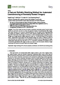
This chapter covers straight block based correlation methods, as iterative methods are not really suitable for real time processing on fast image sequences. First the depth maps of all mentioned cost functions are evaluated by numbers of correct points compared to the ground truth depth map provided within the middleburry datasets. For evaluation of the algorithms the image pairs Art and Dolls from the middleburry stereo data set from 2005 Scharstein (2011) are used. For meeting our test conditions these images were taken in original resolution 1390 x 1110 px and cut to 1024 x 1024 px (See fig. 4). For both datasets the disparity rises up to 220 px.
(a) Art Left Image
(b) Art Brighter
Left
Image
(c) Art Right Image
(d) Art Ground Truth
Fig. 4. Middleburry Stereo Dataset Art Following Scharstein & Szeliski (2002) and Scharstein (2011) the calculation of the depth maps uses 5 x 5 px-blocks while the disparity range is extended to 256 px.
(a) SAD
(b) SSD
(c) ZSAD
(d) ZSSD
(e) ZNCCF
(f) Census
(g) Mini-Census
(h) Ground Truth
Fig. 5. Disparity Maps for various cost functions of the Stereo Dataset Art with unequal exposure time
537
Fast Computation Dense Reliable Depth Maps from Stereo Images Fast Computation of Dense andof Reliable Depth and Maps from Stereo Images
Dataset Art
Dataset Dolls
Cost Function
Equal Exposure
Unequal Exposure
Equal Exposure
Unequal Exposure
SAD SSD
42 % 43 %
0% 1%
51 % 52 %
1% 1%
ZSAD ZSSD
51 % 51 %
34 % 35 %
57 % 57 %
42 % 43 %
ZNCCF 51 % Census 55 % Mini-Census 53 %
41 % 46 % 44 %
55 % 57 % 54 %
50 % 52 % 49 %
Table 1. Accuracy of the Depth Maps for Art and Dolls Depending on the Cost Function While the results of all cost functions of the dataset Art with equal exposure time are very similar to each other, the results for unequal exposure (see fig. 5) show distinct differences. In table 1 the number of correctly estimated points, points with a maximal difference of the disparity value regarding to the ground truth map, are listed for each of the cost functions for equal as well as unequal exposure. The same information is given for the dataset Dolls, yet only in numbers. The best results overall are gained using the Census-transformation, followed by the ZNCCF and the Mini-Census-transformation. The simple SAD and SSD show the worst results. Especially with the unequal exposure these functions are not a good choice. Using the SAD and the SSD cost functions with zero-mean blocks show acceptable results, and when using equal exposure the results are even comparable to the best results of the Census-transformation. The biggest errors of the Census-transformation, the Mini-Census-transformation and the ZNCCF appear at jumps of disparity. These results can be verified by comparing the depth maps with the ground truth data. 3.3 Impact of the block size for correlation
The used block size for the correlation has a major impact on the results. For block based approaches of stereo matching it is assumed that all pixels in a block have the same disparity and the same information is available of both stereo images. The first assumption is violated by all objects which are not aligned parallel to the imaging plane and all blocks with pixel belonging to more than just one object (Faugeras, 1993, p. 191). The second assumption collides with the terms of stereo image acquisition, due to the fact that both images are taken from at least a slightly different angle. Using small block sizes the impact of perspectively distortion and disparity jumps can be minimized while the probability of disambiguation increases. Big block sizes reduce the probability of disambiguation but leads to blurred edges and flattened small details (Kanade & Okutomi, 1991, p. 1). By multiple applications of block based operations, as for the Census-transformation and the correlation, using windowed hamming distance, the effect is amplified (McDonnell, 1981, p. 2). Usually the block size is estimated empirically. Empiric evaluation of the block size for the SAD-function is covered by (Kisacanin et al., 2009, pp. 132) and (Scharstein & Szeliski, 2002, p. 18). Kisacanin et al. (2009) compares the number of incorrect assigned pixels by varying the
54 8
Machine Vision – Applications and Systems Will-be-set-by-IN-TECH
60
8
55
7
50
6
45
5
40
4
35
3
30
Art Dolls Hardware Ressorces
25 20 3x3
5x5
7x7
9x9
11 x 11
13 x 13
15 x 16
17 x 17
2 1
Normalized Hardware Ressources
Correct Disparity Values [%]
block size from 3 x 3 px to 11 x 11 px evincing the result, that the number of errors is decreasing til a block size of 9 x 9 px is reached and is increasing above a block size of 11 x 11 px due to the low pass filter effect of block based methods. (Scharstein & Szeliski, 2002, p. 18) comes to a similar conclusion while the block size here is varied from 3 x 3 px to 29 x 29 px. For two of the three test images the error is at its minimum between 9 x 9 px and 11 x 11 px.
0 19 x 19
Block Size
Fig. 6. Results of the Stereo Matching while Varying the Block Size Compared to the Hardware Resources As the results of both publications are mainly valid for the SAD function, an evaluation for the Mini-Census-transformation was done varying the block size from 3 x 3 px to 19 x 19 px supporting the result of the two publications working with the SAD as the most accurate depth maps here are also calculated using 9 x 9 px and 11 x 11 px for the dataset Dolls. But for the dataset Art the best results are gained by using a block size of 13 x 13 px. The number of errors increases again past the block size of 17 x 17 px. In figures 10(a) to 10(d) in section 4.8 a choice of depth maps is shown in order to visualize the effect of the block size. In 10(a) with a block size of 3 x 3 px the susceptibility of small block sizes regarding to noise is obvious. Due to a large number of incorrect block assignments the objects are almost indistinguishable. Is the block size increased to the maximum of 19 x 19 px the edges are blurred and details of the objects get lost. Using a block size of 9 x 9 px both effects afore mentioned are noticeable but not prevalent. To sum up the results are shown in the diagram in fig. 6 for the datasets Art and Dolls, illustrating that the number of correct block assignments is rising fast for an increased block size with its maximum between the block sizes from 9 x 9 px and 13 x 13 px and falling slowly for bigger block sizes. Additional to the number of correct block assignments for both datasets the diagram shows an estimation for the needed hardware resources. Having squared blocks the hardware resources are rising quadratically. The values are standardized to the needed resources of an hardware implemented stereo analysis for a block size of 7 x 7 px. It is obvious that the stereo image analysis with a block size of 9 x 9 px needs more than one and a half of the resources needed for a block size 7 x 7 px, while the average of the correct block assignment is rising only about 4 % to 5 %. Thus it was decided to use a block size of 7 x 7 px for the processing.
Fast Computation Dense Reliable Depth Maps from Stereo Images Fast Computation of Dense andof Reliable Depth and Maps from Stereo Images
559
4. Methods for improving the reliability of depth maps from stereo images Concluding the above section it becomes obvious that straight block based methods always create incorrect block assignments. To improve the reliability of depth maps, using these methods, requires to identify them as incorrect assignments and exclude their values from further processing steps. The developed methods for improving the depth maps quality are working either iteratively or exclusionary. Iterative methods generate depth maps with higher density and better quality than preclusive methods always resulting in a higher need of computation power, since a lot of intermediate steps have to be calculated as well. Thus the main advantage of excluding incorrect points is that the needed computing power will be reduced, while the main disadvantage is that always correct block assignments are excluded as well. Due to the need of higher computation power iterative methods are not well suited for high speed stereo image processing. The preclusive methods often work with thresholds to keep the processing as simple as possible. Therefore a good algorithm has to be designed in order to mainly exclude incorrect assignments while ideally no correct assignments are excluded. In this section seven known preclusive methods and their parameters are presented, modified and evaluated for maximizing the number of correct points, while minimizing the number of incorrect points in the depth map. The methods discussed in the next section are: maximal disparity, epipolar lines, thresholds on cost function, first absolute central moment as filter for homogeneous regions, the uniqueness constraint, the continuity constraint, left and right consistency check and multi layer correspondence search. All methods are introduced shortly and evaluated for their potential of excluding incorrect assigned blocks. Furthermore the best use cases for each method is determined. 4.1 Physical criteria
The physical constrains can exclude many incorrect candidates for block assignments. The maximal disparity is usually applied in restricting regions of searching for correct block assignments. The same can be done for epipolar conditions. Restricting the area to the epipolar line is easily realized for the normal case of stereophotogrammetry but rather difficult in the standard case of the stereophotogrammetry (Faugeras, 1993, pp. 169). Physical constraints will not be further discussed in this work as they can vary according to the camera setup and the application. The maximum disparity is set to 256. For the epipolar condition the normal case of stereophotogrammetry is used and the search area is reduced to an area parallel to the lines of the image sensor. 4.2 Thresholds on the cost function
The threshold on the cost function can be easily applied to the results of the cost function and is a very common method for improving the reliability. In case of the Census-transformation and the Mini-Census-transformation the hamming distance determines the number of differences between the binary vectors. The results of this test are given in table 2. The threshold of 294 bit is the theoretical maximum of the hamming distance for a 7 x 7 px block and 6 bit Mini-Census vectors. Comparing identical blocks gives a hamming distance of zero. An increasing number of differences between the compared blocks increases the hamming
56 10
Machine Vision – Applications and Systems Will-be-set-by-IN-TECH
distance until the maximum of 294 bit in this case. By applying a threshold to the cost function the maximal difference between both blocks can be limited (Fua, 1993, p. 2). Dataset Art
Dataset Dolls
Maximal Valid Hamming 3-d Points Distance
Correct Correct (Respectively) (Absolute)
Valid 3-d Points
Correct Correct (Respectively) (Absolute)
294 Bit 150 Bit 100 Bit 90 Bit 80 Bit 70 Bit 60 Bit 50 Bit
49 % 49 % 54 % 62 % 70 % 76 % 78 % 79 %
97 % 97 % 90 % 83 % 73 % 61 % 48 % 34 %
57 % 57 % 61 % 65 % 68 % 71 % 72 % 72 %
97 % 97 % 87 % 72 % 54 % 39 % 27 % 17 %
48 % 48 % 47 % 45 % 38 % 30 % 21 % 13 %
55 % 55 % 55 % 54 % 50 % 43 % 35 % 24 %
Table 2. Impact of the Threshold on the Maximal Hamming-Distance on the Correlation Result The calculation of depth maps using various thresholds leads to table 2. All results are given as the ratio of the possible 1048576 point (1024 x 1024 px) in the depth map. The column ”Valid 3-d Points“ represents the rate of the valid 3-d-points. In this case valid 3-d points are identified as valid by applying the threshold on the cost function. The rate of correct block assignments is given by the columns “Correct (Respectively)“ respectively to the valid 3-d points. Correct points show a difference of maximal one pixel for the disparity according to the ground truth. In column “Correct (Absolute)“ the rate of all correct block combinations according to the ground truth depth map is given. Thus it is possible to check how many correct values are excluded. The tables 2 to 7 are setup in the same structure. The results of both images are very similar. Excluding values with a high hamming distance improves the quality of the depth map, by rejecting all points with uncertain matches from the depth map. Yet a very small threshold results in rejecting correct points. In this application a threshold of 90 bits is a good value for restriction via the hamming distance. Here the number of correct points increases about 10% comparing to a threshold of 294 bit (same result when no threshold is given) while only 3% of the correct values are rejected (see table 2). With a threshold of 50 bits for the hamming distance a thin depth map is generated where over 70% of the points are correct according to the ground truth map. The threshold on the hamming distance performs well to rejects incorrect block assignments in case of occlusions due to disparity jumps, but for homogeneous regions its capabilities are limited. 4.3 First absolute central moment for estimating homogeneous regions
Errors in the depth map occur with a high probability in regions of a stereo image pair with low textural information. Especially affected are those areas having the same color or areas covered by large shadows. By identifying blocks belonging to such regions errors can be minimized (van der Mark & Gavrila, 2006, pp. 3). One possibility to identify regions of low texture information is called interest operator,which was introduced by (Moravec, 1977, p. 2) in 1977. The second central moment which complies
Fast Computation Dense Reliable Depth Maps from Stereo Images Fast Computation of Dense andof Reliable Depth and Maps from Stereo Images
57 11
with the variance is calculated in four directions (vertical, horizontal and both diagonals). The minimum of these four values is used as the variance of the block. This interest operator is used in (Konolige, 1997, p.3). Applying the variance σ2 to the whole reference block (Falkenhagen, 1994, p. 4) is another method to estimate areas with low textural information. This is demonstrated in equation (6) for a block at the position i, j of an image. The block size is given by W, in either direction, horizontally and vertically. Il ( x, y) gives the intensity of the pixel at position ( x, y). σ2 =
W
W
1
(2W + 1)
∑
2
∑
k =−W l =−W
( Il (i + k, j + l ) − μ)2
(6)
μ is the average of the intensity and arises from equation (7). μ=
W
W
1
(2W + 1)
∑
2
∑
k=−W l =−W
Il (i + k, j + l ) .
(7)
Calculating the variance, according to equation 6, is not optimized for an FPGA-implementation, due to the number of multiplications and divisions used. While multiplications can be implemented in hardcore embedded multipliers, which are included in most of the current FPGAs, a division is calculated in a resource consuming iterative process (Tornow, 2009, p. 60). To minimize the number of multiplications in a hardware design, the variance known as the second central moment can be replaced by the first absolute central moment (eq. (8)), as used in the opencv library (Willow Garage, 2011, p. 259). In this case the absolute values will prevent that positive and negative differences compensate each other. μ=
W
1
(2W + 1)
2
∑
W
∑
k=−W l =−W
| Il (i + k, j + l ) − μ|
(8)
If the first absolute central moment is applied to blocks of the same size it can be modified, in order to reduce the needed computation power by substituting the term 1/(2W +1)2 with a constant 1/K. Both divisions can be avoided by multiplying the terms in- and outside the summation with the factor K resulting in the equations (9) and (10). With these steps the number of multiplications is reduced to one. μmod =
W
∑
W
∑
k =−W l =−W
μmod =
W
∑
| Il (i + k, j + l ) · K − μmod | W
∑
k =−W l =−W
Il (i + k, j + l )
(9)
(10)
The first absolute central moment was applied to the reference image to identify and exclude blocks with low textural information. Therefore a block size of 5 x 5 px was chosen as this block size is used for the Census-transformation. To extend the block size would mean to increase the memory needed, as only 5 lines of the original image are saved in the FPGA-implementation. Different thresholds were used to reduce the number of incorrect points in the depth map. The results are listed in table 3 as ratio of the maximal number of points in the depth map in the same manner as in section 4.2.
58 12
Machine Vision – Applications and Systems Will-be-set-by-IN-TECH
Dataset Art
Dataset Dolls
Minimal First Valid Absolute Central 3-d Points Moment
Correct Correct (Respectively) (Absolute)
Valid 3-d Points
Correct Correct (Respectively) (Absolute)
0 200 400 500 600 800 1000
49 % 49 % 52 % 54 % 55 % 56 % 56 %
97 % 97 % 95 % 91 % 87 % 79 % 71 %
57 % 57 % 58 % 59 % 60 % 62 % 64 %
97 % 97 % 89 % 83 % 76 % 65 % 57 %
48 % 48 % 46 % 45 % 42 % 36 % 32 %
55 % 55 % 55 % 54 % 52 % 49 % 45 %
Table 3. Impact of the First Absolute Central Moment to the Results of the Correlation Increasing values lead to a higher reliability especially in areas with low textural information. In regions with occlusions this method is not as effective. For the stereo dataset Art, starting with a threshold of 600, a saturation of the reliability can be observed. Increasing the threshold towards higher values will reject correct points. This is not the case for the dataset Dolls. A threshold of 500 in this case, is a good compromise for a dense but reliable depth map as only 1–3% of correct points are rejected, while the reliability is increased by 2–5% . In figures 10(e) and 10(f) the depth maps using thresholds of 500 and 1000 on the first absolute central moment, are shown. The threshold of 500 shows a distinct filter effect in the depth map (see fig. 10(e)). Comparing the depth map with the reference image, it becomes obvious that rejected areas in the depth map correlate with homogeneous colored surfaces in the reference image (see fig. 4(c)). The depth map in fig. 10(f)) shows that the effect of a threshold of 1000 is even stronger. In comparison to fig. 10(e)) the loss of correct block assignments is obvious. 4.4 Uniqueness constraint
The uniqueness constraint was introduced in (Marr & Poggio, 1979, p. 3), it implies that only one disparity value can be assigned to every element of a stereo image. It is substantiated by the physical position of an object which leads to a representation in the reference image and the search image a like alike. Only occlusions by transparent objects violate this constraint (van der Mark & Gavrila, 2006, p. 3). If the first local minimum C1 as well as the second local minimum C2 of the cost function is determined and saved during the correlation process, the uniqueness Cd can be calculated by equation (11). C − C1 Cd = 2 (11) C1 If the clearance between C1 and C2 is small, the uniqueness is small, while the probability of an uncertain result is high. By applying a threshold (see fig 7a) ) multi-assignments can be reduced (Hirschmueller & Scharstein, 2009, pp. 6). Often just the lowest cost function values as shown in fig. 7 are taken for evaluation, due to the complexity of searching for local minima. In this case correct block assignments can be rejected due to a double minima if the eq. 11 (see fig. 7b)) is applied. A double minima
59 13
C3
C3 C1
C1 a)
Hamming-Distance
C2
Hamming-Distance
Hamming-Distance
Fast Computation Dense Reliable Depth Maps from Stereo Images Fast Computation of Dense andof Reliable Depth and Maps from Stereo Images
Disparity
C1 C2
C2
Disparity
b)
threshold
c)
C3
Disparity
Fig. 7. Problem of Double Minima (inspired by Hirschmueller & Scharstein (2009)) occurs if the real minimum is located between two values. To avoid this problem equation 12 compares the first minimum C1 and the third minimum C3 (Hirschmueller & Scharstein, 2009, pp. 6). Uncertain minima are still rejected by this method as shown in fig. 7c). This method performs usually well if the threshold lies between 5 –20 % (van der Mark & Gavrila, 2006, p. 4). C3 − C1 (12) C1 The effect of this method was examined by applying thresholds ranging from 0 % to 25 % to Cd =
Dataset Art
Dataset Dolls
Minimal Valid Distance 3-d Points
Correct Correct (Respectively) (Absolute)
Valid 3-d Points
Correct Correct (Respectively) (Absolute)
0% 2% 5% 7% 10 % 15 % 20 % 25 %
49 % 51 % 57 % 63 % 70 % 80 % 87 % 91 %
97 % 93 % 83 % 76 % 66 % 55 % 47 % 41 %
57 % 59 % 64 % 68 % 74 % 81 % 86 % 89 %
97 % 93 % 79 % 69 % 58 % 44 % 36 % 29 %
48 % 47 % 45 % 43 % 41 % 35 % 31 % 26 %
55 % 55 % 53 % 52 % 49 % 45 % 40 % 36 %
Table 4. Impact of the Uniqueness to the Results of the Correlation the result of the hamming distance, as shown in table 4. By increasing the threshold more correlation results are rejected, while the reliability is increased. In the evaluated range no saturation is reached. A threshold of 7 % gives good results. In Art the reliability increases by 14 % while 5 % of the correct values are rejected. For Dolls the reliability is increased by 11 % while only 3 % of the correct values are lost. In the figures 10(g) and 10(h) depth maps using the uniqueness with a threshold of 7 % and 25 % are shown. Especially in areas of occlusions the multi-assignments could be reduced. The depth map regarding the threshold of 25 % shows reduced errors in regions with occlusions as well as homogeneous regions which result in a reliability of 91 % as listed in table 4.
60 14
Machine Vision – Applications and Systems Will-be-set-by-IN-TECH
4.5 Left right consistency check
A second method based on the uniqueness assumption is the search for corresponding blocks in both directions (Fusiello et al., 1997, p. 2). First suggestion for such a method are sourced in (Cochran & Medioni, 1992, pp. 5) and (Fua, 1993, p. 2) named as Two-View-Constraint and Validity Test. In latter publications (Khaleghi et al., 2008, p. 6) and (Zinner et al., 2008, p. 9) it is called Left-Right-Consistency Checking. Carrying out the search for corresponding blocks two times subsequently with two resulting depth maps Dle f t and Dright is distinctive for this method. In the first run the left image is the reference image, while the right is the search image and in the second run the roles of both images are reversed. The resulting depth maps are very similar but not identical as visible in the figures 10(m) and 10(n) due to the slightly different angle of view of both images (Fua, 1993, p. 2),(Cochran & Medioni, 1992, pp. 5). Afterwards the validation of the correspondence search is realized by crosschecking the disparity. At first the disparity dx_left at the position x and y in the depth map Dle f t is read out and used to determine the position of the corresponding block in Dright . Dright ( x + dx_left , y) = dx_right
(13)
Comparing both disparities gives a clue whether it is a unique block combination. Ideally, regarding the uniqueness assumption the difference between both values has to be zero (Zhao & Taubin (2011)). dx_left − dx_right = 0 (14) The effect of this method was evaluated, by having an implementation where the difference Dataset Art
Dataset Dolls
Maximal Valid Difference 3-d Points
Correct Correct (Respectively) (Absolute)
Valid 3-d Points
Correct Correct (Respectively) (Absolute)
256 px 10 px 3 px 2 px 1 px 0 px
49 % 55 % 56 % 56 % 56 % 56 %
97 % 87 % 85 % 85 % 84 % 80 %
57 % 61 % 62 % 62 % 63 % 62 %
97 % 83 % 81 % 80 % 80 % 77 %
48 % 46 % 45 % 45 % 45 % 43 %
55 % 53 % 53 % 53 % 53 % 50 %
Table 5. Impact of the Left Right Consistency Check on the Depth Maps between both disparity values were be set to any threshold (see. table 5). The number of the points in the depth map as well as the reliability is nearly constant for a difference smaller then 10 pixels and bigger then zero. If a zero-difference between both disparity maps is required a lot of points with a double minima are rejected by this method, hence a threshold of 1 pixel gives the best result as shown in fig. 10(o). 4.6 Applying the continuity constraint
Upon a closer look on a depth map it becomes obvious that incorrect disparity values differ from the neighborhood, especially in homogeneous regions. These nearly homogeneous
61 15
Fast Computation Dense Reliable Depth Maps from Stereo Images Fast Computation of Dense andof Reliable Depth and Maps from Stereo Images
surfaces follow from the continuity assumption which was introduced by (Marr & Poggio, 1979, p. 3) as a continuous run of disparity values named as Continuity Constraint. The Continuity Constraint arises from the usually smooth surface of the objects in a scene. This assumtion is violated at object borders. A similar approach named the No Isolated Pixel Constraint Cochran & Medioni (1992) identifies disparity values as isolated if its difference is bigger than 2.5 px according to the average of a 5 x 5 px-block. This method is evaluated subsequently using a block size of 3 x 3 px. The mean of the difference in the Moore-neighborhood is determined, in order to identify a disparity value as isolated. If the difference of a pixel to its neighborhood is bigger than a threshold it is rejected. Fig. 8 shows two example for a threshold of 30.
150
152
144
151
145
135
144
150
156
150
152
144
151
231
135
144
150
156
mean difference = 6
valid
mean difference = 83
not valid
Fig. 8. Validity of Disparity Values according to the Continuity Constraints The effect of different thresholds using this method is listed in table 6. A decreasing threshold results in a reduced amount of pixels while the rate of correct points in the depth map is rising, since mainly mismatches are rejected. The threshold of 30 is a good choice for keeping a maximum of correct disparity values. Thus the reliability of the depth map rises by 6 % for Art and by 4 % for Dolls whereas only 2 % for Art and 1 % for Dolls of the correct values are lost. The resulting depth map is shown in comparison to depth maps without rejected pixels while not allowing a difference in the figures 10(i) and 10(j). The depth map in fig. 10(i) shows the effectivity of this method, which is able to reject mismatches in homogeneous regions as well as regions with occlusions. Setting the threshold to zero a lot of correct disparity values are rejected as well and the depth map is thinner. The continuity constraint will be used as the final filter in the hardware implementation. It is used for removing isolated pixels, which are left by the other post processing steps as well as outliers in homogeneous regions. While counting the number of valid pixels in their neighborhood it can be easily estimated whether the pixel is isolated or not. Thus in the implementation a pixel identifies as isolated if the number of valid pixels in its neighborhood is less than two, following Cochran & Medioni (1992).
62 16
Machine Vision – Applications and Systems Will-be-set-by-IN-TECH
Dataset Art
Dataset Dolls
Maximal Valid Mean 3-d Points Difference
Correct Correct (Respectively) (Absolute)
Valid 3-d Points
Correct Correct (Respectively) (Absolute)
255 50 40 30 20 10 0
49 % 52 % 54 % 55 % 58 % 63 % 83 %
97 % 93 % 91 % 89 % 84 % 76 % 43 %
57 % 59 % 60 % 61 % 63 % 66 % 84 %
97 % 90 % 87 % 83 % 77 % 66 % 35 %
48 % 47 % 47 % 46 % 45 % 42 % 29 %
55 % 55 % 55 % 54 % 53 % 50 % 36 %
Table 6. Impact of the Continuity Constraint on the Depth Map 4.7 Multi-layer correspondence search
The effect of different sized correlation blocks is described in section 3.3 whereas small block sizes are good for fine details yet sensitive to noise, while big block sizes create a smooth depth map by blurring edges and details. Due to their size big blocks contain more information and have a greater probability for being unique. Thus they can be used to reduce the ambiguity for smaller blocks by checking if the disparity of a smaller block is within a reasonable range. A similar effect can be gained by changing the resolution of the source images. Hierarchical methods are widely used to improve the quality of depth maps or to reduce the computation power. All these methods reduce the resolution of the source images and arrange the resulting images in an image pyramid. A common way is to halve the resolution from layer to layer for implementation reasons (Tornow, 2009, pp. 91). In fig. 9 an example for an image pyramid is given. The correspondence search is carried out with the same block size in all three layers. The information covered by a block rises from layer to layer and complies with the effect of different block sizes (Fua, 1993, p. 5). Yet the implementation is more effective for the coarse layers due to smaller block sizes as well as the reduced image size (Falkenhagen, 1994, p. 1). Nearly all proposed hierarchical methods follow a coarse to fine algorithm, whereas the correlation starts in images with coarse resolution and uses the result as a starting point in the next layer to increase the accuracy. At the second as well as all following layers the range for the disparity search can be reduced to a few pixels. By searching successively throughout all layers the computation power, especially for software implementation can be strongly reduced (Cochran & Medioni, 1992, p. 3), (Sizintsev et al., 2010, pp. 2) and (Zhao & Taubin, 2011, p. 3). Two different approaches are introduced in (Tornow, 2009, pp. 90) and in Tornow et al. (2006). In contrast to the coarse to fine algorithm the disparity search in Tornow et al. (2006) is realized parallel in all layers. Whereas every layer is used to search only in specific non overlapping disparity ranges. This approach shows good results for very large disparity ranges but leads to a coarse resolution for close objects. The proposed approach in (Tornow, 2009, p. 90) complies with the widely used coarse to fine algorithm. Yet it uses the coarse layers to verify the disparity values found in the highest resolutions. Both approaches are well suited for a
63 17
Fast Computation Dense Reliable Depth Maps from Stereo Images Fast Computation of Dense andof Reliable Depth and Maps from Stereo Images
1. layer = 1024 x 1024 px
2. layer = 512 x 512 px
3. layer = 256 x 256 px
Fig. 9. Example of an Image Pyramid hardware implementation. As the method presented in (Tornow, 2009, p. 90) is capable of calculating dense depth maps in hardware it is evaluated in the following. While the block size with 7 x 7 px is constant over all layers, the range for the disparity search is halved layer by layer, starting by 256 px. The resulting disparity maps for layer one is shown in fig. 10(k) and compared to the disparity maps with different block sizes from figures 10(a) to 10(d) the similarity is obvious. If all disparity values, which can not be verified in the next coarse layers, are rejected, the results in table 7 are gained. The threshold for an optimal result is 1 px for Art and 2 px for Dolls. Whereas the improvement of the reliability is about 28 % by having only 1 %–2 % of the correct disparities rejected. This proves the efficiency of the algorithm. Higher thresholds are leading to less reliable disparity maps. Dataset Art
Dataset Dolls
Maximal Valid Difference 3-d Points
Correct Correct (Respectively) (Absolute)
Valid 3-d Points
Correct Correct (Respectively) (Absolute)
256 px 10 px 3 px 2 px 1 px 0 px
49 % 68 % 76 % 79 % 83 % 85 %
96 % 77 % 69 % 67 % 62 % 30 %
57 % 71 % 78 % 80 % 83 % 86 %
96 % 68 % 60 % 58 % 54 % 25 %
47 % 46 % 46 % 46 % 45 % 21 %
55 % 55 % 54 % 54 % 51 % 26 %
Table 7. Impact of the Multi Layer Verification on the Depth Map Comparing the images in figures 10(k) and 10(l) the effect of the method is visualized. Incorrect block assignments are rejected in case of occlusions as well as homogeneous regions.
64 18
Machine Vision – Applications and Systems Will-be-set-by-IN-TECH
The disparity map shown in fig. 10(l) reveals only a few incorrect values and proves the values of table 7. 4.8 Concept of the algorithm
The six presented and evaluated methods for improving the reliability of a disparity map have their strength in different operating ranges. The resulting disparity maps of all methods are shown in fig. 10. The most error-containing regions of an image are regions with homogeneous surfaces and occlusions. Only the multi-layer-verifying performs well for both cases. Mismatches caused by occlusions can be successfully avoided by using the threshold on the hamming distance and the left-right-consistency-check. The first absolute central moment is not suited for treating occlusions. Yet in case of homogeneous regions the minimal hamming distance does not perform well and the first absolute central moment helps avoiding errors in the depth map. The left-right-consistency-check gives average results. The uniqueness constraint and the continuity constraint give moderate results by rejecting incorrect disparity values in both cases. To realize a fast hardware implementation those methods giving the best results, while having the least computation power, should be used. As the hierarchical multi-layer correspondence and the left-right-consistency checking require at least two runs of the correlation process, high computation power is needed. The lowest computation power is used by the minimal hamming distance and the uniqueness constraint. The first absolute central moment and the continuity constraint require an average need of computation power. Parameter
Average
Dense
Reliable
first-abs.-cen.-moment max. hamming-distance uniqueness constraint continuity constraint
500 90 Bit 7% 30
400 100 Bit 2% 50
800 70 Bit 15 % 10
Art – valid 3-d-points
40 %
70 %
15 %
correct (respectively) correct (absolute)
84 % 34 %
64 % 45 %
95 % 14 %
Dolls – valid 3-d-points 54 %
80 %
26 %
correct (respectively) correct (absolute)
67 % 54 %
93 % 24 %
82 % 44 %
Table 8. Results Using Different Setups As the threshold on the hamming-distance and the uniqueness can successfully reject a lot of mismatches, the results, especially in homogeneous regions, are not good enough, thus the first absolute central moment and the continuity constraint are added to the set of post-processing. In table 8 three sets of used thresholds and the achieved results of the two stereo data sets are given. The three different parameter sets are suitable to provide disparity maps with different attributes. The dense-setup gives a low reliability of about 60 % with a big amount of
65 19
Fast Computation of Dense and Reliable Depth Maps from Stereo Images
Fast Computation of Dense and Reliable Depth Maps from Stereo Images
(a) Mini-Census 3 x 3 px (b) Mini-Census 7 x 7 px (c) Mini-Census 9 x 9 px (d) 19 x 19 px
(e) 1st-Abs.-Cen.-Mom. (f) 1st-Abs.-Cen.-Mom. 500 1000
(i) Continuity 30
(j) Continuity 0
(m) Dle f t
(n) Dright
(g) Uniqueness 7 %
(k) Layer 1
(o) Left-Right-Cons.-Check
Mini-Census
(h) Uniqueness 25 %
(l) Multi-Layer-Approach
(p) Ground Truth
Fig. 10. Depth Maps of Middleburry Stereo Datasets Art Using Various Method for Improvement
66 20
Machine Vision – Applications and Systems Will-be-set-by-IN-TECH
3-d-points. The average- setup with a reliability of more than 80 % is suitable for the most common applications, such as interactive robots, driver assistance systems, facial detection etc. The reliable-setup is capable of providing disparity maps with over 90 % reliability and is therefore suitable for safety systems. Applying these four post-processings very good results of the multi-layer correspondence search are surpassed by using less hardware resources. In some applications it is more important to have a very dense depth map therefore a certainty value to each 3-d point is added. In such a case the certainty for a 3-d point can be estimated using the methods for quality improvement presented in the sections 4.3 to 4.7 as measurement tools to weight the impact of 3-d-points. In this case fine graduation would give very dense depth maps without any loss of information.
5. FPGA-implementation Having evaluated all processing steps for a fast, reliable stereo image analysis, suitable for hardware implementation, the next step was to generate a modular and fully platform-independent design using VHDL. 1., 2., 3. Minimum and Disparity reference block Hammingsearch block
Minimum
Distance
a stage Delay
Minimum
HammingDistance
Delay
Hamming-
Minimum
1. and 3. Min., Disparity
Distance
frame, line-, block number,
Delay
first central moment
frame, line, block number, first central moment
Fig. 11. Structure of the Cascaded Correspondence Analysis The design is divided into preprocessing, the correlation process and post processing. The preprocessing contains the calculation of the first absolute central moment and the Census-transformation of the stereo image pair, using a block size of 5 x 5 pixels and the determination of the frame-number, line-number and block-number of the synchronization signals. Currently no further filter processes are included. The correlation process is set up by a cascade of processes calculating the hamming distance and determining its first and third minimal value, as shown in fig. 11. The number of blocks for which the hamming distance is calculated in such a stage depends on the required processing speed. For very high speed processing only one block combination of the hamming distance is calculated per stage. The number of stages can be determined by dividing the maximal disparity by the number of hamming distances calculated per stage. For high speed calculations with a disparity range
Fast Computation Dense Reliable Depth Maps from Stereo Images Fast Computation of Dense andof Reliable Depth and Maps from Stereo Images
67 21
of 256 pixels, when only one block combination is processed per stage, 256 stages are needed. If only a lower speed is required, for example 16 block combinations can be processed in one stage, thus only 16 stages are needed.
(a) Aloe D:71 % R:89 % (b) Baby3 D:42 % R:80 % (c) Books D:40 % R:77 % (d) Dolls D:55 % R:84 %
(e) D:35 % R:73 %
Laundry (f) D:55 % R:91 %
Moebius (g) Reindeer (h) D:56 % R:84 % D:81 % R:93 %
Rocks1
Fig. 12. Depth map of Different Datasets of the Middlebury Stereo Dataset (D: Density – Rate of Valid Pixels; R: Reliability – Rate of Correct Disparity Values) In the post processing the four chosen methods of improvement the reliability of the depth map are applied: Starting with the first absolute central moment, followed by the uniqueness constraint and the maximal hamming distance, ending with the continuity constraint. The last step of the post processing is to calculate the depth map from the disparity map using equation (2) according to the calibration information. Using Alteras NIOS-II processor the processing can be compiled as a hardware coded function available from within the processor. Thus small sets of block combinations could be processed on demand by the processor. The configuration was tested with a Terasic DE3-board containing an Altera Stratix III EP3SE260 using a set of PhotonFocus cameras MV-D1024 Photonfocus (2008) connected via CameraLink-interface. Using the hardware implementation the datasets Aloe, Art(D: 44 % R: 80 %), Baby3, Books, Dolls, Laundry, Moebius, Reindeer and Rocks1 of the Middlebury stereo dataset were processed (see fig. 12) using the parameter set average. The overall density is 53 % and the overall reliability is 84 %. Correct points show a difference of maximal one pixel for the disparity regarding the ground truth.
6. Comparison with the state of the art of stereo image analysis systems An implementation on different FPGA-platforms could be realized due to a fully platform independent design. In table 9 five different versions are listed. The implementations for the Virtex 6, the Stratix IV and the Cyclone III, which are marked with an *, were only tested with
68 22
Machine Vision – Applications and Systems Will-be-set-by-IN-TECH
a timing simulation. Just the implementations using Stratix III was tested on real hardware. The hardware approach introduced in section 5 is running with a disparity range of 256 px at a maximal pixel clock of 189 MHz on an Altera Stratix III FPGA. With an image size of 1024 x 1024 px a frame rate of 180 Hz could be reached. Reference
Hardware Platform
Hirschm. & Scharst.(2009) CPU – 2,6 GHz Xenon Zinner et al. (2008) CPU – 2,0 GHz Core 2 Duo Sizintsev et al. (2010) Zhao & Taubin (2011)
GPU – GeForce GTX 280 GPU – GeForce GTX 280
Khaleghi et al. (2008) Chang et al. (2007)
DSP – ADSP-BF561 DSP – TMS320C6414T-1000
Jin et al. (2010) Pelissier & Berry (2010) Masrani & MacLean (2006) Zhang et al. (2011) This work This work This work This work This work
FPGA – Virtex 4 FPGA – Cyclone III FPGA – Stratix FPGA – Stratix III FPGA – Stratix III FPGA – Stratix III FPGA – Stratix IV* FPGA – Virtex 6* FPGA – Cyclone III*
Image Size
Max. Frame Disparity Rate
450 x 375 px 450 x 375 px
64 px 0.5 fps 50 px 13 fps
640 x 480 px 1024 x 768 px
256 px 32 fps 256 px 36 fps
160 x 120 px 384 x 288 px
30 px 20 fps 16 px 50 fps
640 x 480 px 1024 x 1024 px 640 x 480 px 1024 x 785 px 1024 x 1024 px 1024 x 1024 px 1024 x 1024 px 1024 x 1024 px 1024 x 1024 px
64 px 64 px 128 px 64 px 256 px 64 px 256 px 256 px 180 px
230 fps 160 fps 30 fps 60 fps 180 fps 205 fps 198 fps 241 fps 124 fps
Table 9. State of the Art of Stereo Image Analysis Systems (* Only Timing Simulation) A comparison with state of the art implementations on major platforms for on-line processing is shown in table 9. By comparing different approaches it has to be taken into account, that every platform has its own advantages and disadvantages. PC-based solutions are generally used when the focus lies on the quality of the depth map or when the frame rate is not important. The approach of Hirschmueller & Scharstein (2009) provides a slow processing speed, but with a high accuracy. It covers a comparison of several different methods. Zinner et al. (2008) is optimizing a PC-based software implementation, it reaches 13 Hz while the maximum disparity is 50 px. This article shows clearly that image size and disparity range are a trade off to the frame rate. Both approaches use rather small image sizes. DSP based solutions (Khaleghi et al. (2008) and Chang et al. (2007)) for the stereo image analysis are even more limited on image size and disparity range as well as their frame rate. Due to DSPs which are optimized for processing one dimensional signals. Image processing on DSP is still important for smart phones. The proposed algorithm is suitable for GPU-implementation as well, but the Census-transformation is optimized for hardware implementation. Thus the different cost functions should be used. For high speed applications massive parallelizing is necessary. This can be realized either by hardware implementation or using SIMD-processors, as used in current GPUs. The advantage of GPUs is the possibility of high speed processing with at least double precision floating point units, using a high speed memory connection. Furthermore GPUs can be programmed using standard programming languages like C and are fairly cheap. On the other hand some of the cheap GPUs are limited in accuracy, due to their main field of application as graphic cards.
Fast Computation Dense Reliable Depth Maps from Stereo Images Fast Computation of Dense andof Reliable Depth and Maps from Stereo Images
69 23
While rendering images is an easy task on GPUs, optimizing other algorithms to GPUs is still a difficult task. Sizintsev et al. (2010) uses an adaptive coarse to fine algorithm and a left right consistency check. The system is capable of a frame rate of 32 Hz on images with a resolution of 640 x 480 px, while the disparity range is 256 px wide. By skipping some parts of the algorithms for the sake of improving the quality, 113 Hz are possible. The overall rate of points with a higher difference to the ground truth than one pixel is 15.8 %. The approach of Zhao & Taubin (2011) reaches 36 Hz with an algorithm optimized to measure moving parts in stereo images. After using a foreground detection a multi-resolution stereo matching is applied. The overall error rate lies by 14.5 %. Generally GPUs are capable of calculating dense and reliable depth maps, yet the power consumption and the waste heat of GPU based systems are a major draw back for usage in embedded systems. Nevertheless the combination of small GPUs with embedded microprocessors are on their way. FPGAs are well suited for embedded systems as they have a very low power consumption combined with a high processing speed. Programming FPGAs is a time consuming process which requires special knowledge, regarding digital electronics and hardware programming. The implementation of complex iterative algorithms in FPGAs is possible but it is often less effective, as FPGA implementations are data flow driven with concurrent processing of algorithm parts. Thus iterative algorithms which provide depth maps with the highest quality must be highly adapted as they are heavily control flow oriented. Straight algorithms perform very well on FPGAs due to their data flow orientation. The quality of the disparity maps in the presented work is, with 84 %, in the same dimension as other state of the art FPGA-solutions. The rate of incorrect points in the depth map ranges from 14 % in Zhang et al. (2011) to 17 % in Jin et al. (2010). The hardware resources required are fairly low compared to other approaches. Zhang et al. (2011) requires about 95000 logic blocks and 3.77 MBit of memory at the Stratix III, compared to ca 40000 logic blocks and 321 kBit of memory needed for the presented solution with a disparity range of 64 px (disparity range of 256 px used for this research (⇒ ca 147000 logic blocks and 328 kBit). The approach presented by Jin et al. (2010), implemented on a Virtex 4, needs 51000 logic elements and 322 memory blocks compared to the Virtex 6 implementation with a disparity range of 64 px with 39000 logic elements and 23 memory blocks (disparity range of 256 px ⇒ ca 149000 logic blocks 23 memory blocks). Both approaches provide more dense disparity maps due to a more complex post processing but with a lower disparity range. Only the Cyclone III implementation of Pelissier & Berry (2010) requires 61000 logic blocks and 131 kBit which are less than the 72000 logic blocks and the 322 kBit of memory needed by our approach, yet without post processing for improving the depth map quality and a disparity range of 64 px.
7. Conclusion In this chapter an algorithm for generating dense and reliable disparity maps of stereo images, suitable for high speed processing, using an FPGA, is presented. Therefore several cost functions, as well as post processing steps to increase the reliability, are evaluated. The algorithm uses a correlation with the hamming distance, having a block size of 7 x 7 px, on Census transformed images. In four post processing steps incorrect points of the disparity map are rejected and the reliability as well as the quality is increased up to 84 % of correct pixels for the average-setup. By choosing a set of parameters either a very dense or a very
70 24
Machine Vision – Applications and Systems Will-be-set-by-IN-TECH
reliable (reliable-setup: 95 % reliability) depth map can be calculated. Due to its modular setup the implementation can be easily adapted for optimizing either speed or needed FPGA-resources. In Stratix III the implementation runs with a maximal frame rate of 180 Hz, having a resolution of 1024 x 1024 px and a disparity range of 256 px. The main applications for high speed stereo analysis are autonomous robots and driver assistance systems as well as in line quality controls and sensor systems for automation. Especially for grid based analysis of the surroundings, used for vicinity observations for autonomous vehicles and driver assistance systems, a dense and reliable depth map can be provided. Hence the problem of splitting one object into several objects due to the low resolution of the depth map can be overcome. This method can be adapted to be well suited to various applications due to a modular setup where processing speed, which is not needed, can be easily used to reduce the size of the implementation. Additional post processing steps, iterating on the results given by the presented algorithm, could increase both, the reliability and the density of the depth map, while requiring more hardware resources as well.
8. References Albertz, J. & Wiggenhagen, M. (2009). Guide for Photogrammetry and Remote Sensing, 5. edition edn, Wichmann. Bay, H., Andreas, Ess, A., Tuytlaars, T. & Gool, L. V. (2008). Surf: Speeded up robust features, Computer Vision and Image Understanding(CVIU), Vol. Vol. 10, pp. pp. 346–359. Chang, N., Lin, T.-M., Tsai, T.-H., Tseng, Y.-C. & Chang, T.-S. (2007). Real-time DSP implementation on local stereo matching, Proceedings of the IEEE International Conference on Multimedia and Expo, pp. p. 2090–2093. Chang, N. Y.-C., Tsai, T.-H., Hsu, B.-H., Chen, Y.-C. & Chang, T.-S. (2010). Algorithm and architecture of disparity estimation with mini-census adaptive support weight, IEEE Transactions on Circuits and Systems for Video Technology Bd. 20(6): pp. 792–805. Cochran, S. D. & Medioni, G. (1992). 3-d surface description from binocular stereo, IEEE Transactions on Pattern Analysis and Machine Intelligence Bd. 4(10): pp. 981–994. Falkenhagen, L. (1994). Depth estimation from stereoscopic image pairs assuming piecewise continuos surfaces, Proceedings of the European Workshop on Combined Real and Synthetic Image Processing for Broadcast and Video Production, pp. 115–127. Faugeras, O. (1993). Three-Dimensional Computer Vision : A Geometric Viewpoint, MIT Press, Cambridge, MA. Favaro, P. & Soatto, S. (2007). 3-D Shape Estimation and Image Restoration, Springer-Verlag. Fua, P. (1993). A parallel stereo algorithm that produces dense depth maps and preserves image features, Machine Vision and Applications Bd. 6(1): pp. 35–49. Fusiello, A., Roberto, V. & Trucco, E. (1997). Efficient stereo with multiple windowing, Proceedings of the 1997 Conference on Computer Vision and Pattern Recognition (CVPR ’97), pp. 858–863. Hirschmueller, H. & Scharstein, D. (2009). Evaluation of stereo matching costs on images with radiometric differences, IEEE Transactions on Pattern Analysis and Machine Intelligence Bd. 31(9): pp. 1582–1599. Jin, S., Cho, J., Pham, X. D., Lee, K. M., Park, S.-K., Kim, M. & Jeon, J. W. (2010). FPGA design and implementation of a real-time stereo vision system, IEEE Transactions on Circuits and Systems for Video Technology Bd. 20(1): pp. 15–26.
Fast Computation Dense Reliable Depth Maps from Stereo Images Fast Computation of Dense andof Reliable Depth and Maps from Stereo Images
71 25
Kanade, T. & Okutomi, M. (1991). A stereo matching algorithm with an adaptive window: Theory and experiment, Proceedings of the 1991 IEEE International Conference on Robotics and Automation (ICRA ’91), Vol. 2, pp. 1088–1095. Khaleghi, B., Ahuja, S. & Wu, Q. M. J. (2008). An improved real-time miniaturized embedded stereo vision system (mesvs-ii), IEEE Computer Society Conference on Computer Vision and Pattern Recognition Workshops (CVPRW ’08), pp. 1–8. Kisacanin, B., Bhattacharyya, S. S. & Chai, S. (2009). Embedded Computer Vision, Springer-Verlag, London. Konolige, K. (1997). Small vision systems: Hardware and implementation, Proceedings of the International Symposium on Robotics Research, pp. 111–116. Marr, D. & Poggio, T. (1979). A computational theory of human stereo vision, Proceedings of the Royal Society of London. Series B Bd. 204(1156): pp. 301–328. Masrani, D. K. & MacLean, W. J. (2006). A real-time large disparity range stereo-system using FPGAs, in P. Narayanan, S. Nayar & H.-Y. Shum (eds), Computer Vision - ACCV 2006, Vol. 3852, Springer-Verlag, Berlin Heidelberg, pp. 42–51. McDonnell, M. (1981). Box-filtering techniques, Computer Graphics and Image Processing Bd. 17(1): pp. 65–70. Moravec, H. (1977). Towards automatic visual obstacle avoidance, Proceedings of the 5th International Joint Conference on Artificial Intelligence, p. 584. Narasimha, R. (2010). Depth Recovery from Stereo Matching Using Coupled Random Fields, PhD thesis, UNIVERSITÃL’ DE GRENOBLE. Pelissier, F. & Berry, F. (2010). Design of a real-time embedded stereo smart camera, in J. Blanc-Talon, D. Bone, W. Philips, D. Popescu & P. Scheunders (eds), Advanced Concepts for Intelligent Vision Systems, Vol. 6474, Springer-Verlag, Berlin Heidelberg, pp. 344–356. Photonfocus (2008). User manual – MV-d1024 series CMOS area scan cameras, Online-Source. Scharstein, D. (2011). Middlebury stereo datasets, Online-Source. URL: http://vision.middlebury.edu/stereo/data Scharstein, D. & Szeliski, R. (2002). A taxonomy and evaluation of dense two-frame stereo correspondence algorithms, International Journal of Computer Vision Bd. 47(1): pp. 7–42. Sizintsev, M., Kuthirummal, S., Samarasekera, S. & Kumar, R. (2010). GPU accelerated realtime stereo for augmented reality, Proceedings of the 5th International Symposium 3D Data Processing, Visualization and Transmission (3DPVT ’10). Szeliski, R. (2010). Computer Vision : Algorithms and Applications, Springer-Verlag, London. Tornow, M. (2009). Untersuchung und Entwicklung von Algorithmen zur Stereobildauswertung fuer die Erfassung von Objekten im Umfeld von Fahrzeugen und Realisierung einer Hindernisdetektion in Echtzeit mittels einer Hardwareimplementierung auf einem FPGA, Dissertation, Otto-von-Guericke-University, Magdeburg. Tornow, M., Kazubiak, J., Kuhn, R. W., Michaelis, B. & Schindler, T. (2006). Hardware approach for real time machine stereo vision, Journal of systemics, cybernetics and informatics Bd. 4(1): pp. 24–34. Trucco, E. & Verri, A. (1998). Introductory Techniques for 3-D Computer Vision, Prentice Hall, Upper Saddle River, NJ. van der Mark, W. & Gavrila, D. M. (2006). Real-time dense stereo for intelligent verhicles, IEEE Transactions on Intelligent Transportation Systems Bd. 7(1): pp. 38–50. Willow Garage (2011). The opencv 1.x c reference manual, Online-Quelle.
72 26
Machine Vision – Applications and Systems Will-be-set-by-IN-TECH
Zabih, R. & Woodfill, J. (1997). A non-parametric approach to visual correspondence, IEEE Transactions on Pattern Analysis and Machine Intelligence. Zhang, L., Zhang, K., Chang, T. S., Lafruit, G., Kuzmanov, G. K. & Verkest, D. (2011). Real-time high-definition stereo matching on FPGA, Proceedings of the 19th ACM/SIGDA international symposium on Field programmable gate arrays (FPGA ’11), pp. 55–64. Zhao, Y. & Taubin, G. (2011). Real-time stereo on GPGPU using progressive multi-resolution adaptive windows, Image and Vision Computing Bd. 29(6): pp. 420–432. Zinner, C., Humenberger, M., Ambrosch, K. & Kubinger, W. (2008). An optimized software-based implementation of a census-based stereo matching algorithm, Advances in Visual Computing, Vol. 5358, Springer-Verlag, Berlin Heidelberg, pp. 216–227.