Fuzzy Control of a Multivariable Nonlinear Process A. Iriarte Lanas1, G. L.A. Mota1, R. Tanscheit1, M.M. Vellasco1, J.M.Barreto2 1 DEE-PUC-Rio, CP 38.063, 22452-970 Rio de Janeiro - RJ, Brazil e-mail: 1(ricardo, marley)@ele.puc-rio.br;
[email protected] Abstract
2: Description of the Plant This paper presents a qualitative control of a fluid mixer, which is a multivariable and intrinsically non-linear plant. The mixer has as inputs two fluids of different colours and the output is the colour of the resulting mix. The control system consists of two independent fuzzy controllers which are responsible for maintaining the water level at a given height and for adjusting the colour of the fluid in the mixing tank. The main points studied are the response when the desired colour is changed and when the output flow changes. Simulation results show that the approach of using two independent controllers, with simple rule-bases, can give good results.
1: Introduction Ordinary fuzzy controllers have been succesfully applied to a variety of plants since the pioneering works of Mamdani and colaborators [1]. In the case of multivariable processes, the natural approach would be to consider as rules antecedents all the controller inputs, which grow in number as the number of desired outputs, or reference inputs, grows. This would certainly make the process of designing the control strategy, or rule-base, a more complex one. On the other hand, if independent controllers are used for each reference input, rule-base design becomes simpler and the control strategy becomes potentially more reliable. In the case of robot control through a learning fuzzy controller [2], it has been shown that the use of independent controllers for each link can give good results. That is, the controllers, by adjusting their set of rules, cope very well with the coupling between variables. In this work the approach of using separate fuzzy controllers is employed, with the purpose of verifying whether this strategy is adequate. The plant, described in the next section, is a fluid mixer, which, by presenting non-linear characteristics, provides an additional complexity and constitutes a good test for the designed fuzzy control system.
The plant, shown in Fig.1, consists of a mixing and two auxiliary tanks. The first auxiliary tank contains coulored water c1, while the second one contains clear water c2. The input flow q to the mixing tank is controlled by two valves, which regulate the output flows q1 and q2 from the auxiliary tanks. The output flow q0, taken as a disturbance, has the coloration c of the resulting mix and is a function of the output pipe cross-section ab, of the liquid level h in the mixing tank and of a constant Cd related to the shape and material of the output pipe. In oder to simplify the simulation, it has been assumed that the auxiliary tanks always contain sufficient liquid for the process to keep on running. The mixing tank dimension is 20x10x180 cm. and the output cross-section ab can be set to values between 0 and 0.4 cm2. The output flow q0 lies between 0 and 60 cm3/sec. Colorations c1 and c2 are set to 1 and 0, respectively.
Fig. 1: The Fluid Mixer To derive a mathematical model, so that a simulated experiments can be performed, the time needed to obtain a uniform mixture, time delays related to flows in the pipes and the dynamics of input and ouput valves have been neglected [3].
The following equations model the plant dynamics: dV dh = S. dt dt q = q1 + q 2
q - q0 =
(1)
q 0 = Cd.ab.
(2) (3)
2gh
where g is the gravity acceleration, V is the volume of liquid and S is the area of the liquid surface in the mixing tank. By using (3) in (1): Cd.ab. 2gh q dh =− + dt S S
(4)
The mixing process is modelled by: dh 1 = (q1 + q 2 − q 0 ) dt S d(c0 .S.h) dh dc c1.q1 − c 0 .q 0 = = S.(c0 . + h. 0 ) dt dt dt
(5) (6)
By combining (5) and (6): dc 0 1 = .(c1.q1 − c 0 (q1 + q 2 )) dt Sh
(7)
Equations (4) and (7) describe the system's dynamics; h and c0 are the variables to be manipulated by the controlling system.
3: Fuzzy Control System The control strategy is described by a set of linguistic statements, or rules. Consider, for example, the case where each control rule relates two input variables e and ce to the controller ouput u, and a control algorithm consisting of a set of rules R1, R2,..., Rn, of the IF (E is Ej) AND (CE is CEj) THEN (U is Uj) form, connected by a ELSE connective [4]. The combination of those rules can be expressed mathematically (by its membership function) as: µRN (e,ce,u) = f1[µR1 (e,ce,u), ...., µRn (e,ce,u)]
(8)
where f1 expresses the ELSE connective. In (8) above, each control rule j can be expressed as: µRj (e,ce,u) = f2 [f3 (µE (e), µCEj (ce)), µUj (u)] j
(9)
In (9), E = {e}, CE = {ce}, U = {u} are finite universes and Ej, CEj and Uj are fuzzy subsets of those universes. The operator f2 stands for implication [5], and f3 is the interpretation of the connective AND, which is
usually taken as min (∧). The controller decides which action to take through a compositional rule of inference. As is generally the case in control, the controller inputs are real measured values given by singletons, and called here es and ces. The controller output fuzzy set Us will thus be given by: µUs(u) = f1[f2 (µE1(es) ∧ µCE1(ces), µU1(u)), ... ...., f2 (µEn(es) ∧ µCEn(ces), µUn(u))]
(10)
Since the process requires at its input non-fuzzy values, the controller output fuzzy set must be defuzzified, the result being a value us. In the fluid mixer under consideration, the control system has to be designed to keep both the output coloration c0 and the liquid height h in the mixing tank at desired setpoints. The quantitative information needed by the control system in order to attain those goals is given by the coloration error ec and change in error Δec, the height error eh and the ouput flow q0. Since the chosen strategy makes use of two independents fuzzy controllers, one for height control and another for coloration control, it is more convenient to choose as output variables the total flow q (equation 2) and the proportion qr of coloured water in the total flow, defined as: q1 (11) qr = q1 + q 2 The height controller has two quantitative inputs, eh and q0, and one ouput, q. The coloration controller has as quantitative inputs ec and Δec, and as its ouput Δqr. There is a slight difference between the height and coloration controllers. While in the former precision is not a fundamental factor, in the latter the goal is to have a fine control, with null steady-state error if possible; thus the use of a structure with PI characteristics.
3.1: Height Control In the design of the height controller, fuzzy sets NB, NM, Z, M, B, PB are assigned to Eh={eh}, and fuzzy sets Z, S,M, B, VB to Q = {q} and Q0 = {q0} , as specified by their membership functions shown in Fig. 2 and Fig. 3 below. The universes of discourse for each variable are clearly shown in those figures. The non-fuzzy actual values of the measured input variables are mapped to the chosen universes of discourse through scaling factors GEh and GQ0, which are part of blocks S0 and S1 in the simulation diagram of Fig. 6. The resulting values are called ehs and q0s. The defuzzified controller output qs is mapped to the process input actual values through a scaling factor GQ, so that q = qs x GQ. In this controller, f1 is implemented by max and f2 by min; Mean of Maxima (MOM) [6] is used for defuzzification.
Fig. 2: Membership functions for Eh
Fig. 3: Membership functions for Q and Q0 The rule-base for height control is summarized in Table I, where the entries correspond to the values of Q.
Eh
Q PB PM Z NM NB
Z M S Z Z Z
S M B VB B VB VB VB M B VB VB S M B VB Z S M B Z Z M B
Fig. 5: Membership functions for ΔQr
The larger number of fuzzy sets used for the controller output in coloration control, as compared to height control, is due to the requirement of higher accuracy in the coloration of the resulting mix than that for the level of liquid in the mixing tank. In fact, the reason for keeping h at a desired setpoint is mainly to prevent an undesirable overflow in that tank. The rule-base for coloration control is summarized in Table II, where the entries are the values of ΔQr.
Q0 Table I: Rule-base for height control
3.2: Coloration Control In the coloration controller, fuzzy sets NB, NB, Z, PM and PB are used for Ec={ec} and ΔEc={Δec}, while fuzzy sets NVB, NB, NM, NS, Z, PS, PM, PB and PVB are used for the controller output ΔQr={qr}, as specified by their membership functions shown in Fig. 4 and Fig. 5. The universes of discourse are as shown in those figures. The actual measured values of the controller inputs are mapped to the universes of discourse through scaling factors GEc and GΔEc, (contained in S2 and S3 in the diagram of Fig. 6), the result being variables ecs and Δecs. The defuzzified controller output Δqrs is mapped to the process input actual values through a scaling factor GΔQr. The actual input flows to the fluid mixer are given by q1=qr×q and q2=qr−q1. In this controller, f1 is implemented by max, and f2 by product [6]; defuzzification is performed through Centre of Gravity (COG), which in general provides smoother responses than MOM. Fig. 4: Membership functions for Ec and ΔEc
Ec
ΔQr NB NM Z PM PB Z PB NVB NB NM NS Z PS PM NB NM NS Z PS PM Z NM NS Z PS PM PB NM NS Z PS PM PB PVB NB ∆Ec Table II: Rule-base for coloration control
4: Simulated experiments The process response will depend on the scaling factors, which can be empirically set beforehand and then tuned in order to improve the controller performance. For example, in the case of the fluid mixer, the range established for q and q0 was from 0 to 60 cm3. Since the corresponding universes of discourse are [0,4], GQ and GQ0 were initially set at 15. This value gave origin to satisfactory responses and did not need to be tuned. The maximum possible height error eh was assumed to be ± 7 cm, which, considering the corresponding universe as [-2,2], gives GEh=0.3. In order to have good accuracy in coloration, and by noting that the universe of discourse is [-2,2] for that variable, the scaling factor GEc was
eventually set at 200; GΔEc was set at 1500. Finally, GΔQr was made equal to 1/15. In the simulation MATLAB, its associated tool SIMULINK and the FuzzyToolbox have been used. The simulation diagram is shown in Fig. 6. Experiment 1: The resulting mix coloration behaviour for output valve settings of 0.1, 0.2 and 0.4 cm2 is shown in Fig. 7, when a step from 0.1 to 0.3 is applied to the reference input. The level of liquid in the mixing tank should be kept constant 30 cm. It can be seen that the larger the output valve opening, the faster the change in coloration. Since the level of liquid must be kept unchanged, the larger the output flow, the larger the input one, which causes a faster change in coloration. It can be
concluded that the coloration controller tries to reach the reference input as fast as possible, but this will also depend on the action of the height controller on the input flow. Experiment 2: The level (height) of liquid in the mixing tank is shown in Fig. 8 when a step from 10 to 50 cm is applied to the height reference input. Output valve settings of 0.1 and 0.2 cm2 have been used.; the final coloration should be kept unchanged at 0.5. It can be observed that in both cases the reference is quickly achieved, but the control is not as precise as in the coloration case. As said before, this is due to less rigid specifications for height control. The objective of keeping coloration unchanged at 0.5 was also achieved.
Fig. 6: Simulation Diagram
0.1 0.2
0.4
0.2
0.1
Fig. 7: Experiment 1
Fig. 8: Experiment 2 Experiment 3: Coloration and height variations are shown in Fig. 9 for different output valve openings when steps of
0.1 to 0.3 and of 0 to 30 cm. are apllied to the coloration and height reference inputs, respectively. It can be observed that the reponse-time is smaller than in experiment 1. This can be attributed to a larger input flow, since the step applied to the height reference input allows a rather fast change in coloration. The response shows a small overshoot and the output valve opening has a small influence on the overall behaviour.
The tuning of the controllers showed, as expected, that the system's performance is sensible to changes in the scaling factors. Although this is beyond the scope of this work, an automatic tuning procedure could be of help in this respect. This same plant is being used for further investigations, such as automatic rule creation and modification and the design of a MIMO fuzzy controller, with four inputs and two outputs. Results will then be compared to those presented in this work.
6: References
Fig. 9: Experiment 3
5: Conclusions The simulated experiments have shown that the approach of using two independent fuzzy controllers in the control of a MIMO system can give good results. In the plant considered in this work, the introduction of a new variable allowed the reasoning process to occur in a decoupled fashion. The main objective of reaching a specified coloration for the liquid in the mixing tank was achieved with very good precision - error of less than 0.001. The height controller was capable of maintaining the liquid level in the mixing tank near the reference value, even without the use of the change in error as a controller input.
[1] Mamdani, E.H., "Application of fuzzy algorithms for control of simple dynamic plant". Proc. IEE (Control and Science), V. 121, pp. 1585-1588, 1974. [2] Tanscheit, R. and Lembessis, E., "On the behaviour and tuning of a fuzzy rule-based self-organising controller". In: Mathematics of the Analysis and Design of Process Control. P. Borne, S.G. Tzafestas, N.E. Radhy (Eds). Elsevier Science Publishers, 1991. [3] Barreto, J.M., Hierarchical Control of Fluid Mixer". Ciência e Técnica (Brazil) , V. 13, pp 35-39, 1976. [4] Lembessis, E. and Tanscheit, R., "The influence of implication operators and defuzzification methods on the deterministic output of a fuzzy rule-based controller". Proc. 4th IFSA Congress, Brussels, 1991. [5] Mendel, J.M. “Fuzzy logic systems for engineering: a tutorial”, Proc. IEEE, V. 3, pp. 345-376, 1995. [6] Driankov, D.; Hellendorn, H.; Rheinfrank, M., "An Introduction to Fuzzy Control". Springer-Verlag, 1993.
Acknowledgement This work was partially supported by the Brazilian Research Agencies CAPES and CNPq.