Oct 28, 1980 - Lebedev [7], and Stroud [13, Sections 2.6 and 8.4]. The methods discussed in the present paper are not optimal, but they are well-suited to the ...
J. Austral. Math. Soc. (Series B) 23 (1982), 332-347
NUMERICAL INTEGRATION ON THE SPHERE KENDALL ATKINSON
(Received 28 October 1980) (Revised 1 February 1981)
Abstract
This is a discussion of some numerical integration methods for surface integrals over the unit sphere in R3. Product Gaussian quadrature and finite-element type methods are considered. The paper concludes with a discussion of the evaluation of singular double layer integrals arising in potential theory.
1. Introduction
This is a discussion of some numerical integration methods for the surface integral / ( / ) = / AQ)do, (1.1) J u with U the unit sphere in R3. The integration formulae will include product Gaussian quadrature and some methods based on breaking U into smaller triangular elements with various associated low order integration schemes. The motivation for discussing such methods arises from the desire to solve integral equations defined over simple smooth surfaces S in R3, Xp(P) - f K{P, Q)p(Q) da(Q) = +(P),
P e S.
(1.2)
Such equations can arise in a variety of applications, although we are particularly interested in those equations arising from solving potential theory problems in R3. To deal with integrals over a general surface S, we assume there is a smooth 1-1 mapping of U onto S; then an integral over S can be transformed into one of the form (1.1). © Copyright Australian Mathematical Society 1982. 332
[2 ]
Numerical integration on the sphere
333
The product Gaussian quadrature formula is discussed and illustrated in Section 2. Methods for triangulating the sphere and some associated integration formulas are given in Section 3. Since most kernel functions K(P, Q), in (1.2), are singular in potential theory applications, we discuss the evaluation of one such integral in Section 4. For a review of integration methods on the sphere, see Keast and Diaz [6], Lebedev [7], and Stroud [13, Sections 2.6 and 8.4]. The methods discussed in the present paper are not optimal, but they are well-suited to the solution of integral equations. Moreover, the theory of optimal methods is far from complete, as has been noted in [7]; consequently it would not be possible to carry out a complete error analysis of the resulting numerical methods for solving (1.2). 2. Product Gaussian quadrature
Let /(/) be written using spherical coordinates / ( / ) = F'
fW F{9, ) sin 0 dB d,
(2.1)
•'o •'o with/(0, ) =f(x, y, z). The integral is approximated by 1m
4(/) = ^ 2
m
2 " , M , ,)•
(2.2)
The {0,} are chosen so that (cos(0,)} and {tv,} are the Gauss-Legendre nodes and weights on [-1, 1]. The points ty are evenly spaced on [0, 2m\ with spacing •n/m; usually j=jv/m
or
\j - ^ U/m.
(2.3)
With this choice of node points and weights, Im{f) integrates exactly any polynomial f(x, y, z) of degree less than 2m; see [13, page 40] for a proof. For an integration formula, the degree of precision is n if the formula is exact for some polynomial of degree n + 1. Hence Im(f) has degree of precision 2m — 1. The formula Im(f) is less efficient than the optimal formulae of [7], but not badly so. For methods of an increasing degree of precision, Lebedev introduces the efficiency index ),
(2.4)
where n is the degree of precision and N(n) the number of associated node points on if. The larger the index for a given n, the more efficient is the method. The formulae developed by Lebedev satisfy ij(n) -» 1 as n -» oo. The above Gaussian formula has index ij(2m — 1) = 2/3 for m > 1. Lebedev's formulae use only 2/3 the number of node points used by Im(f). This is not a large difference and it is offset somewhat by the ease with which Im(f) is constructed.
Kendall Atkinson
334
[3]
Convergence results for Im(f) can be obtained from an approximation theorem of Ragozin [11]. Using this, it is straightforward to show that, if f(x,y, z) is k times continuously differentiable on U, then for m > 1. (2.5) |/(/) - Uf)\ < Cl ((2m - l)k) This bound shows the same rapid convergence associated with Gaussian quadrature for one variable integration. A short proof of (2.5) is given in [1]. EXAMPLES. Four numerical examples will be given, and they will be referenced by the four different surfaces 5, that are used. The first two examples are
f ex da,
i = 1, 2,
(2.6)
with S, the ellipsoidal surface (x/a)2 + (y/b)2 + (z/cf = 1, where 5, uses (a, b, c) = (1, 1, 2) and S2 uses (1, 2, 5). The last two examples are to calculate the surface area of 5,,
f da,
J
s, with S, a 'peanut-shaped' region given by (x,y,
i = 3, 4,
z) = R(6) (a cos sin 9, b sin sin 9, cos 9)
where
R(9) =[cos(20) +[c - sin 2 (20)] 1/2 ]' /2 .
Figure 1. Cross-section of the ellipsoid S2-
(2.7)
[4]
Numerical integration on the sphere
335
Figure 2. Cross-section of the surface S3.
Figure 3. Cross-section of the surface St.
Surface 5 3 uses (a, b, c) = (1, 2, 2) and S4 uses (1, 2, 1.1). The cross-sections in the x, z-plane of the surfaces S2, S3, and 5 4 are shown in Figures 1 to 3. Surfaces 5"2 and S4 are somewhat more ill-behaved than 5, and S3. Table 1 contains the numerical results for the four integrals. The column n gives the number of integration nodes. As expected, the convergence is rapid.
Kendall Atkinson
336
[s]
TABLE 1
Errors for product Gaussian quadrature Relative error for the integration over 5, m
n
4 8 12 16 20
32 128 288 512 800
i =1
/=2
i-3
-3.0E-4 -1.3E-6 -9.0E-9 O.0E-12 s m c e t n e triangulation 7],M is needed to obtain the nodes used in Jn(f).
340
Kendall Atkinson
[9]
TABLE 5
Numerical examples 1 and 2 for the isoparametric method Surface S, Nodes
Relative error
20
62
-2.8E-2
80
242
-2.OE-3
n
Surface S2
Ratio
Relative error
Ratio
-3.0E-2 14.3
13.7 -2.1E-3
16.0
15.3 320
962
-1.3E-4
-1.3E-4
TABLE 6
Numerical examples 3 and 4 for the isoparametric method Surface S3 n 20
Nodes
Relative error
62
-3.2E-2
Surface S4
Ratio
Relative error -1.8E-1
31
11 80
242
-2.9E-3
320
962
-1.3E-4
Ratio
-5.8E-3 -6.9
12 8.4E-4
Based on our examples, the centroid rule should be used in preference to the isoparametric method /„(/), provided n is not too large and Tin is used. With other values of n or other triangulations, /„(/) is much more competitive, and possibly superior. Comparing with the other examples for the product Gaussian quadrature, the latter is generally superior in accuracy to C n (/), especially at moderate to high error tolerances. ERROR BOUND DERIVATIONS. We will give only a sketch of the proof of (3.9); the details are straightforward, but algebraically complicated. First, note that the integration rule (3.8) is exact for all polynomials g(s, I) of degree < 3. For a general differentiable function g(s, t), an error formula can be found in the standard way: expand g(s, t) in a Taylor series through the third degree plus a remainder term, and apply the error functional for (3.8) to this equation. The error will be proportional to the fourth derivatives of g.
I io 1
Numerical integration on the sphere
341
To apply this to deriving (3.9), first assume that f(x,y, z) is defined in a neighborhood of U, with continuous and bounded fourth order derivatives. Since (3.8) is applied to (3.7), consider the fourth derivative of the integrand in (3.7). It can be shown that 34
, t))\q, X q,\] , - t>3|6}. (3.10)
In addition, the following results can be shown for our triangulations Tt „, To „, and Tun: cjn < Area(A,) < c 2 /2, for i = 1, . . . , n, (3.12) where c, and c2 > 0 and independent of n; furthermore, c3 max{|c, - v2f, \v2 - v3\2, \v3 - t>,|2} < Area(A,) < c4 min{|t>i - v2\2, \v2 - v3\2,\v3 - u,| 2 },
(3.12)
with i = 1, . . ., n, u,, v2 and v3 the vertices of A,, and c3 and c4 > 0 independent of n. Combining all of these results with the error formula for (3.8), derived using a Taylor series, we obtain (3.9). For functions f(Q) defined only on U, if they are four times differentiate using a local parametrization on U, then they can be extended to a new function on a neighborhood of U; and the extensions can be chosen to have the same degree of differentiability. For a discussion of this, see [4, pages 13, 100]. The proof of (3.5) is quite similar. We write >-/(&)Area(A,)
M*. 0)1* x q,\ as * - \j[q{\, I))|,,(I, I) x q,{\, I 2 = £/'> + E?>.
(3.13)
The point ( \ , 3 ) is the centroid of o0, and Q, = q{ y , 3 ). The integration rule /
g{s,t)dsdt~)rg(\,\)
(3.14)
has degree of precision 1. Using the same kind of proof as that given for (3.9), it follows that P = O(l/n2).
(3.15)
342
Kendall Atkinson
[ 111
For ZT/2), repeat the same argument, with g(s, i) = \qs X q,\ in (3.14). Using the boundedness o f / o n U, we obtain £,(2) = 0(1/n2). Thus Ei = O(l//i 2 ), and the sum of the errors over {A,} is O(\/n).
4. Evaluation of a singular integral The use of integral equations in the solution of potential theory problems in R3 leads to the evaluation of singular surface integrals; for example, see Jaswon and Symm [5]. As an example of the treatment of such integrals, we will consider the evaluation of
f d(B)
dv(A)
with S a smooth boundary surface for a simply connected region, v(A) the inner normal to S at A, and d(B) a smooth density function (called the double layer density). This integral arises from the representation of harmonic functions as double layer potentials in R3; the singularity in (4.1) is of order \/\A — B\. Unfortunately, there does not seem to be any way to remove the singularity using a change of variables, and it must be treated directly. There is another formulation in terms of solid angles: for example, see Mikhlin [10, page 349], but that too has significant problems when trying to calculate the solid angles, especially when B is near to A. As before, assume there is a 1-1 mapping of U onto S and then use it to change the integral in (4.1) to one over U. This leads to the integral operator %p(P) = f K(P, Q)p(Q) da(Q), P&U. (4.2) J u The kernel K includes the original kernel of (4.1) and the change of the surface area differential. A PRODUCT GAUSSIAN known identity
QUADRATURE FORMULA.
Begin by applying the well-
to obtain %p(P) = 2-np(P) + f
K(P, Q)[P(Q) - p(P)] da.
(4.3)
The new integrand is bounded at Q = P, although it will still be discontinuous.
Numerical integration on the sphere
343
If we were now to change to spherical coordinates for Q, then the point P would become a singular point internal to the integration region [0, w] X [0, 2m\. Most numerical integration methods perform poorly in such a situation, and that will be true here. To avoid this, we first rotate the coordinate system, Q' = HQ, (4.5) with H a Householder orthogonal matrix. It is to be chosen so that P' = HP is (0, 0, 1) or (0, 0, -1). We use a spherical coordinates representation for Q', and apply the product Gaussian quadrature with respect to this new representation. The singularity in the integrand occurs along either 0 = 0 or 9 = n. This change of variables results in much improved accuracy and, moreover, there is now a regular behaviour to the error as the integration parameter m is increased. (1) We choose S = U and, to have a test case, use the result that %p = 2ir/(2k + l)p, for k > 0, for any spherical harmonic of degree k. (See [9, page 69] for the definition of spherical harmonics). We choose the spherical harmonics EXAMPLE.
pm(P) = z and p(2>(P) = z2 - (x2 + y2)/2.
(4.6)
For P, we have (-.30353, .93417, .18759).
(4.7) 2
The index of integration is m, and the number of nodes is n = 2m . The numerical results are given in Table 7. TABLE 7
Gaussian rule: example 1 for singular integral m
n
Error for %pw
4
32
1.4E-3
8
128
2.0E-4
16
512
2.7E-5
32
2048
3.5E-6
Ratio
Error for SCp(2)
Ratio
-1.0E-2 7.1
6.9
-1.4E-3 7.4
7.4
-1.9E-4 7.7
7.7
-2.5E-5
(2) We use the surface S3 with the density functions of (4.6) and let P be the point on 5 3 corresponding to the point of (4.7) on U, P = (-.20036, 1.23330, .12383). The errors in Table 8 were calculated using a very accurate value of %p(P), obtained with a much larger value of m.
Kendall Atkinson
344
[13]
TABLE 8
Gaussian rule: example 2 for singular integral m
n
Error for 9Cp(1)
4
32
-5.2E-2
8
128
-5.7E-4
16
512
-5.4E-5
32
2048
-7.2E-6
Ratio
Error in DCp