... orthogonal neural net- work which, due to its structural analogy to fast algorithm ... Fast Orthogonal Neural Networks, Image Recognition,. Signal and Image ... work training and they solve it with a convolutional neural network based on the ...
FAST ORTHOGONAL NEURAL NETWORK FOR ROTATIONTRANSLATION- AND SCALE-INVARIANT IMAGE RECOGNITION
ABSTRACT In this article a novel method of image recognition invariant under rotation, translation and scaling is presented. The proposed method is based on a fast orthogonal neural network which, due to its structural analogy to fast algorithm for Fourier amplitude spectrum computation, enables to classify images irrespectively of their translations. This property, in conjunction with log-polar representation of image amplitude spectrum, is subsequently applied to obtain also the rotation and scale invariance. The proposed classifier is compared to a multilayer perceptron and to k-nearest neighbors method, showing its superiority in a series of tests performed on specially constructed image databases. KEY WORDS Fast Orthogonal Neural Networks, Image Recognition, Signal and Image Processing
1
Introduction
The problem of invariance is one of the key issues in Image Recognition (IR) applications. Determining which visual aspects of an object make it belong to a certain class and which may vary within classes may be a difficult, problemspecific task. Affine transformations such as rotation or scaling are often considered unimportant when we think of object recognition, so we usually try to build some intermediate image representation, suitable for passing to the classifier, which would be invariant under those transformations. This process, which may be subdivided into image registration phase and feature extraction phase, is crucial for proper operation of the classifier as most classifiers are generally highly sensitive to image registration errors. Therefore, the classification results depend on finding the parameters of possible affine transformations of the recognized object and, most notably, finding the object itself, which may impose significant difficulties in the case of real-life images containing other objects and noisy background. Considering the fact that successful segmentation and analysis of complex scenes is still a problematic task, it is worth considering a question: could a classifier itself be invariant to affine transformations of unregistered images? We are interested in raw image classification, which may seem difficult due to high dimensionality and redundancy of the input data, but which at the same time eliminates the risk of losing some possibly discriminative information while building an intermediate representation of
an image. An interesting analysis and validation of this approach was presented in [1] on the example of MNIST database of handwritten digits. LeCun et al. emphasize the shift-invariance problem in the context of neural network training and they solve it with a convolutional neural network based on the idea of replicating the neural weight configuration across space. In this work we propose a different approach: we use an analogy to shift invariance property of Fourier amplitude spectrum [2] [3] to obtain a neural network invariant to input image translation. In contrast to typical approaches in which Fourier amplitude spectrum of an image is computed and some of its coefficients then form a fixed feature vector for a classifier [4] [5], we use a fast orthogonal neural network (FONN) to compute the spectrum in an adaptable way. The whole classification system consists of a single, multilayer neural network in which the input layers provide the shift invariance property, as their sparse connection scheme is based on fast algorithm of Fourier transform, and the output layer computes and assigns the final class labels. In this way we do not have to determine which spectral coefficients are important and should be included in the feature vector. Moreover, although the FONN part of the system may learn the exact amplitude spectrum values, it may also learn other transforms, possibly preserving the phase information. This information, rejected in a typical approach based on amplitude spectrum only, may be used to further enhance classification results.
2
The Principles of Fast Orthogonal Neural Networks
Fast orthogonal neural networks (FONN) are linear, feedforward neural networks with a specific architecture based directly on fast algorithms of orthogonal transforms [6] [7]. They consist of O(logN ) layers, each containing typically N/2 neurons, where N is the size of input/output vectors. Each neuron, is a simple processing unit (Basic Operation Orthogonal Neuron, BOON) with two inputs and two outputs, corresponding to a single basic operation of the original fast algorithm. The distinguishing property of the FONN is that the fixed coefficients of a basic operation of a fast algorithm become adaptable weights of the corresponding BOON. The BOONs may contain four independent weights for an arbitrary 2 × 2 linear operation [8]: � � � � y1 v1 = P· , (1) y2 v2
Figure 1. Neural representation of the basic operation P4
Figure 2. a) Element computing absolute value; b) Computational scheme
3
where �
w11 w21
P = P4 =
w12 w22
� ,
(2)
(this is equivalent to two independent “classical” linear neurons with two inputs, Fig. 1), but they may also contain two or, ultimately, only one weight: � P2 =
u −w
w u
�
� ,
P1 =
1 −t
t 1
� .
(3)
The application of the BOONs based on the matrices P2 , P1 instead of P4 is possible due to the orthogonality of basic operations of the original fast algorithm. In this way we obtain two-fold or four-fold reduction of the number of neural weights. The adaptation of a FONN is based on the following formulas defining the components of the gradient vector and the error vector for a single BOON [7]: "
∂E ∂u ∂E ∂w
"
#
� =
(n−1)
e1 (n−1) e2
v1 v2 #
"
(n−1)
e1 (n−1) e2
" P2T
·
−v1
�
=
� ∂E = v2 , ∂t
� " (n) # e1 · , (n) e2
v2 −v1
(n)
e1 (n) e2 "
#
· "
=
P1T
·
# ,
(n)
e1 (n) e2 (n)
e1 (n) e2
(4)
(5)
# ,
(6)
# ,
(7)
where P T denotes the transpose of P . The parameters v1 and v2 represent the inputs of the h iT (n) basic operation, the vector e(n) refers to the , e 2 1 error values propagated back from the next layer and the h iT (n−1) vector e(n−1) defines the error values to , e2 1 be propagated back from the current layer to the previous one. The formulas (4) - (7) have a general meaning, i.e. they are applicable to a basic operation irrespective of its location in the network architecture. Moreover, no specific architecture is imposed as the information about the indexes of the interconnected basic operations’ inputs/outputs is sufficient. Given the components of the gradient vector, any known gradient method may be successfully applied to minimize the error function of the network [7] [4] [9].
FONN-based Image Recognition
As it was mentioned in section 1, the proposed system consists of two main parts: the FONN based on a fast algorithm of Fourier transform and the output layer. In order to let the FONN part compute the Fourier amplitude spectrum, a special layer of amplitude-computing elements must be appended to it [10] (Fig. 2 a). Training of the neural network containing elements from Fig. 2 a) is based on the following observations: the elements of this type do not have weights, therefore the size of the gradient vector remains the same; the value of error signal passing through this element during backpropagation must be adequately modified. In order to compute the modified value of error signal let us consider the scheme presented in Fig. 2 b). It contains two basic computational blocks: the block corresponding to our neural network and the block representing the error function. Both blocks are connected via the element computing the absolute value. Taking into account the following: q � fi2 (w) + fj2 (w) , (8) u(w) = the value of error signal with respect to the weights vector is given as: � � ∂E ∂E ∂u ∂E 1 ∂fi ∂fj = = 2fi + 2fj = ∂w ∂u ∂w ∂u 2u ∂w ∂w ∂E fj ∂fj ∂E fi ∂fi + . (9) = ∂u u ∂w ∂u u ∂w Hence, the target modification of error values during backpropagation amounts to multiplying them by the quotient input/output of the elements under consideration [10]. Let us now consider the two-dimensional Fourier transform, defined for a discrete two-dimensional signal x(n, m) as [11] [8]: XN ×M (p, q) =
N −1 M −1 X X
pn
qm
x(n, m)e−j2π N e−j2π M , (10)
n=0 m=0
where j is the imaginary unit, p, n = 0, 1, ..., N − 1 denote the row number, q, m = 0, 1, ..., M − 1 denote the column number, and N , M define the height and width of the input image, respectively. The fast algorithm for computing Eq. (10) is based on fast homogeneous two-stage algorithm [12] of cosine transform, type II [13]: LII N ×M (p, q) =
N −1 M −1 X X
(2n+1)p
x(n, m)C4N
(2m+1)q
C4M
,
n=0 m=0
(11)
4
through the following relation [14]: pM +qN Re{XN ×M (p, q)} = LII + T (p, q)C4N M
Experimental Validation and Discussion
4.1
pM +qN pM +qN LII + LII − T (p, M − q)S4N M T (N − p, q)S4N M pM +qN LII , T (N − p, M − q)C4N M pM +qN Im{XN ×M (p, q)} = LII − T (p, q)S4N M pM +qN pM +qN LII − LII − T (p, M − q)C4N M T (N − p, q)C4N M pM +qN LII , T (N − p, M − q)S4N M
(12) pM −qN Re{XN ×M (N − p, q)} = LII − T (p, q)C4N M pM −qN pM −qN II II LT (p, M − q)S4N M + LT (N − p, q)S4N M + pM −qN LII , T (N − p, M − q)C4N M pM −qN Im{XN ×M (N − p, q)} = −LII − T (p, q)S4N M pM −qN pM −qN II II LT (p, M − q)C4N M + LT (N − p, q)C4N M − pM −qN LII , T (N − p, M − q)S4N M k k = sin (2πk/K); Re, Im = cos (2πk/K), SK where CK are the real and imaginary parts of a complex number, respectively, and LII T denote the result of the transform (11) computed for input signal x(n, m) subjected to the following permutation:
xT (2n, 2m) = x(n, m) , xT (2n + 1, 2m) = x(N − 1 − n, m) , (13) xT (2n, 2m + 1) = x(n, M − 1 − m) , xT (2n + 1, 2m + 1) = x(N − 1 − n, M − 1 − m) . The resulting graph of the complete neural image recognition system, including the amplitude-computing layer and the output layer is presented in Fig. 3. Naturally, considering the recursive nature of the fast cosine transform algorithm [12] it is possible to apply Eq. (12) to obtain a classifier for input of size N × N for any N being a power of 2. The number of neurons in the last layer corresponds to the number of classes. The error function is defined as the mean square error between the obtained output vector and the target vector having all zeros except of the position corresponding to the number of the expected class, set to “1”. The connections denoted with (*) need additional explanation. They are simple one-to-one connections, without any adaptable coefficients, which need a trivial modification of backpropagation procedure. They are not necessary for amplitude spectrum computation, which is ob2 tained from the first N2 + 2 outputs of the same layer (note that due to Fourier spectrum symmetry for real images [11] this is exactly the number of relevant spectral elements). However, during experiments involving phase information retrieval it was observed that they significantly enhance classification. Although the network was able to use the phase information for image recognition without those connections, which we find an interesting property, adding them enabled to reach even more pronounced results.
Translation Invariance
Our primary goal is to show that the proposed network may classify objects irrespective of their position in an image. This is to be contrasted with typical applications of neural networks in which the input should be carefully registered [5]. A multilayer non-linear perceptron has been initially chosen for comparison [4] [9], but it appeared quite unsuitable for the analyzed test cases, mainly due to long training phase and difficulty in selecting the proper number of hidden neurons. Since a comparison with a standard KNN classifier [15] showed, after many experiments, that the latter yields similar (in most cases better) results, we decided to present only exemplary MLP results obtained for one of the tests with several numbers of hidden units. In all the other test cases the KNN classifier, with the number of nearest neighbors K = 1, has been applied instead. Three test image databases: T1, T2 and T3 have been constructed in order to verify the translation invariance property of the proposed network. For this purpose several objects in a fixed position have been chosen from the COIL database [16] (Fig. 4). • T1: This database contains 4 objects (classes) of the same size and orientation presented on black background in random positions. • T2: This database contains 2 objects of the same size and orientation presented on black background. Each object is used to construct two classes: in one class it appears in random positions on the right half of the image and in the second class it appears on the left half. • T3: This database is constructed in the same way as T2, but the objects are presented on background obtained by cutting a square fragment from a different image (classic Fishing boat image). Each database was generated several times with different number of training images to assess the generalization properties of the classifier. One hundred testing images were used in all cases and the validation dataset size was set to one-fourth of the training set (rounded up to the nearest integer). The initial size of all the images was set to 128 × 128. However, as it was found that the size 32 × 32 was sufficient, yielding similar results, the images were downscaled using bilinear interpolation before feeding them to the classifier. The resulting 1024-element input vectors were normalized and the constant component was removed. The comparison between the FONN and the KNN results for the T1 database is presented in Fig. 5. Figure 6 shows the result obtained with the MLP classifier for 50 training images per class (200 in total) with different number of hidden neurons. All the presented values (except of
Figure 3. The complete neural architecture for input images of size 4 × 4 and two target classes
Figure 4. The class representatives (three images per class) in databases T1, T2, T3
Figure 7. Classification results (T2 database)
Figure 5. Classification results (T1 database)
Figure 8. Classification results (T3 database)
Figure 6. MLP classification results for 50 training images per class (T1 database)
the KNN classifier outcomes) are mean results obtained after ten-fold repetition of the training phase from a random starting point in the weights space. Apart from the classification results of the MLP which are significantly lower than those of the KNN (81.4% for 32 hidden units vs. 91.8%, respectively), the training process was also slow and prone to get stuck for long periods. The minimum of the validation error curve was usually reached after several hundred epochs. In contrast, the FONN classifier needed only 61 epochs on average to reach the 100% recognition rate on the validation set. It should be stressed that both neural networks were tested in the same conditions, including input/target values, adaptation method and parameters (off-line learning with conjugate gradient algorithm and directional minimization based on 3rd order polynomial approximation [4]). It is also worth noting that the recognition rate on the training dataset was 100% for both networks in all the cases, including the smallest training set of 5 images per class. Therefore, the FONN results presented in Fig. 5 may be interpreted in terms of the generalization error. A simple solution to translation invariance problem is to analyze the Fourier amplitude spectrum instead of the raw image. Indeed, the KNN easily reached the classification of 100%, even with 5 images per class when image amplitude spectra were used as input. The same result was obtained within 2-5 epochs for the FONN classifier working with raw images, but with the initial weights values set
according to the Fourier transform algorithm. The superiority of our “adaptive Fourier transform” may be easily shown when the phase information has to be also taken into account. Obtaining classification over 50% of the T2 set based on amplitude spectrum only is impossible, as the images from classes 1, 3 and from classes 2, 4 have equal amplitude spectra. In contrast, the FONN classifier may take advantage of both its translation invariance property and adaptation potential. The results shown in Figures 7, 8 confirm high classification potential of the proposed classifier, which is best seen when objects are presented on noisy background (recognition on raw images from T3 database for 300 training objects per class: 93.6% for FONN vs 73.8% for KNN). 4.2
Rotation, Translation and Scaling Invariance
Rotation and scaling of an image may be reduced to translation if we change the image coordinate system from cartesian to log-polar via the log-polar transform (LPT) [3] [2]. The difficulty which cannot be neglected here is that the initial image should not be shifted, as even small translations may give huge differences of the log-polar representation. Therefore, a method of providing shift invariance must be applied first. Spatial-domain techniques based on e.g. center of mass, shape or contour coefficients [3] [5] significantly depend on the segmentation process which may be imperfect for real-life images. The alternative is to use amplitude spectrum of the original image, which is known to be shift-invariant and it also preserves image rotation and
Figure 11. Classification results (RTS1 database) Figure 9. a) Image amplitude spectrum; b) Log-polar representation
scaling (with inverse of the scaling coefficient). Expressing Fourier amplitude spectrum in log-polar representation (FFT-LPT) yields shift invariance and changes the rotation and scaling into translations (Fig. 9) [2]. Obtaining the complete rotation, translation and scaling invariance (RTS invariance) using the log-polar representation of the amplitude spectrum is possible in a similar way we obtained the translation invariance in section 4.1 using raw image representation. We can therefore compute the Fourier amplitude spectrum again (FFT-LPT-FFT) and perform classification or apply the FONN classifier for the same purpose. In the following part of this section we will compare these two methods showing the advantages of the approach based on FONN with respect to KNN classifier. Three test image databases: RTS1, RTS2 and RTS3 have been constructed in a similar way to the databases T1, T2 and T3 (Fig. 10). • RTS1: This database contains 4 different objects (classes) presented on black background. The images within each class are varied by rotation angle from the range (0°, 360°), scale coefficient from the range (0.9, 1.5) and position. • RTS2: This database contains 2 objects. Each object is used to construct two classes: in one class it is rotated by a random angle from the range (-30°, +30°) or (150°, 210°), which means in practice “roughly vertical position”; in the other class the angles are taken from either of the ranges (60°, 120°) or (240°, 300°), which yields “roughly horizontal position”. Besides, the scale coefficient and position are varied exactly as in the RTS1 database. • RTS3: This database is constructed in the same way as RTS2, but the background is obtained similarly to the T3 case. The testing procedure was the same as in the case of T1 - T3 with the exception that for every input image of size 128 × 128 Fourier amplitude spectrum of the same size was computed and it was transformed to the log-polar representation of size 32×32. This representation was normalized and fed to the classifier, exactly as the raw image was in section 4.1.
Two details are worth noting here. Firstly, due to Fourier symmetry property for real signals [11] only half of the amplitude spectrum is significant. Therefore, the logpolar sampling was actually set to produce 64 × 32 representation which was afterwards cut by half to the final size of 32 × 32. Secondly, prior to normalization, the intensity of the obtained representation was transformed by logarithm function in order to increase the dynamic range of high frequency components [5]. The comparison between the FONN and the KNN results for the RTS1 database is presented in Fig. 11. Two additional results have been shown here, apart from those based on the discussed representation (FFT-LPT) with the FONN (light gray) and the KNN classifier (dark gray). These are: KNN classifier performing recognition on the same data representation as in the case of the T1 - T3 databases, i.e. on raw images (black) and KNN classifier using the Fourier amplitude spectrum of the discussed representation (FFT-LPT-FFT, white). The latter test shows that for well-segmented objects the non-adaptable, fully RTS-invariant approach yields good results. However, for a more complicated case when the phase information must be also taken into account this method definitely fails. The databases T2 and T3 are constructed in such a way that a shift of the FFT-LPT representation along the vertical axis, corresponding to rotation of the spectrum and - at the same time - of the original image, cannot be neglected. In this case, only operating on FFTLPT representation enables to perform correct recognition, which is shown by the KNN (FFT-LPT) and FONN classifiers. However, the important difference between them is that the FONN does provide the shift invariance, due to its structural analogy to the algorithm for Fourier amplitude spectrum computation, which does not exclude using also the phase information. In contrast, the KNN is a statistical method, which can “simulate” shift invariance if given sufficient training data, as it was shown in section 4.1, but it is basically unaware of the underlying model of affine transformations. The results obtained for the RTS2, and especially for the RTS3 databases (Figures 12 and 13) seem to confirm this reasoning. The FONN recognition rate for 50 training images with noisy background per class (69.56%) is comparable with the result the KNN method can offer for 300 training images (67.8%). Using 300 images with the FONN classi-
Figure 10. The class representatives (three images per class) in databases RTS1, RTS2, RTS3
Figure 12. Classification results (RTS2 database)
Figure 13. Classification results (RTS3 database)
fier enables to reach the recognition rate of 85.06% which seem to be a good result for this particular dataset. Analyzing the obtained results it is worth to consider the proposed classification method in a wider context. The databases T1 and T2 would present an easy, almost trivial task for most existing image recognition systems, especially when the shift invariance and the relevance of object position in the T2 database would be manually set up. Note, however, that general classification methods would not easily and automatically adapt to changes in location of objects, which was shown on the example of the KNN and MLP classifiers. Successful segmentation of the objects from the T3 database would be problematic due to many details present in the background. A possible approach would explore correlation techniques [5], which would probably be successful, yielding additionally the position of an object within an image. The drawback of correlation is that it assumes matching every object against the analyzed image, which may be slower than simply forwarding the input image through the FONN (which requires a comparable number of arithmetic operations to the FFT algorithm). For example, performing correlation in the frequency domain, which may be more efficient for bigger images, still needs computing the inverse FFT for every template (i.e. for every class) and finding the global maximum of the correlation function. On the other hand, the FONN is a neural network so it must be trained, which may take some time. Nevertheless, this is the price we pay for compact representation (the vector of weights; cf. the data needed by the KNN method), efficient operation in the recognition phase and adaptability potential, which the correlation-based methods may lack. It should be also stressed that the presented classifier works directly on training images, needing no additional knowledge, such as explicit templates to match.
The databases RTS1 and RTS2 may be successfully classified with statistical methods, assuming the knowledge of the underlying affine transformation model. The RTS3 database, however, seem to present quite a difficult classification task. The observations made for the T3 database hold true also in this case, with an exception that the direct correlation will inevitably fail. An effective but inefficient solution would be to apply exhaustive search through all possible values of the rotation angle and scale coefficient, which would turn out to be a very time-consuming process. In this context the presented FONN-based solution seems to be an interesting alternative, especially when the recognition speed and robustness is important.
5
Conclusion and Future Work
In this paper a fast orthogonal neural network has been applied to construct a classifier suitable for raw image analysis and recognition. The presented classifier enables to successfully recognize objects in images without the need of image registration, segmentation, edge detection or other typical preprocessing techniques. The classifier has been compared to other methods on several databases designed for testing the rotation-, translation- and scale-invariance. Special attention has been paid to verify that it can also make use of the phase information when necessary, which distinguishes it from most methods based on amplitude spectrum representation. Indeed, although the proposed classifier is actually based on the RTS-invariance model, it was shown to perform successful image recognition even when this model is deliberately violated by a given task explicitly setting the shift information as discriminative. In this paper the problem of translation invariance has been tested separately from the other two affine transformations. This approach is justified by the novelty of the proposed tool which had to be examined on the more elementary level first. It is however possible to apply the fast orthogonal neural network both for the raw images, to obtain translation invariance in an adaptable way, and again for the log-polar representation as it was done here. Replacing also the fixed log-polar transform with a linear layer having a suitable connection scheme would yield a neural architecture of interesting properties. Our future work will explore this possibility, indicating potential application areas.
References [1] LeCun, Y., Bottou, L., Bengio, Y., Haffner, P.: Gradient-based learning applied to document recognition. Proc. of the IEEE, vol. 86(11), pp. 2278–2324 (1998) [2] Milanese, R., Cherbuliez, M.: A rotation-, translation, and scale-invariant approach to content-based image retrieval, J. Visual Comm. Image Rep. 10, pp. 186– 196, (1999)
[3] Derrode, S., Ghorbel, F.: Robust and Efficient FourierMellin Transform Approximations for Gray-Level Image Reconstruction and Complete Invariant Description. Computer Vision and Image Understanding 83, pp. 57–78 (2001) [4] Osowski, S.: Neural networks for information processing. (in Polish) OWPW, Warsaw (2000) [5] Gonzalez, R.C., Woods, R.E.: Digital Image Processing, 2nd Edition, Prentice-Hall Inc. (2002) [6] Jacymirski, M., Szczepaniak, P.S.: Neural realization of fast linear filters. In: Proc. of the 4th EURASIP - IEEE Region 8 International Symposium on Video/Image Processing and Multimedia Communications. pp 153–157 (2002) [7] Stasiak, B., Yatsymirskyy, M.: Fast Orthogonal Neural Networks. ICAISC 2006. LNAI, vol. 4029, pp. 142– 149. Springer Verlag (2006) [8] Szczepaniak, P.S.: Intelligent computations, fast transforms and classifiers. (in Polish) EXIT Academic Publishing House, Warsaw (2004) [9] Rutkowski, L.: Methods and techniques of artificial intelligence. (in Polish) Polish Scientific Publishers PWN (2005) [10] Stasiak, B., Yatsymirskyy, M.: Fast orthogonal neural network for adaptive Fourier amplitude spectrum computation in classification problems. In Proc. of the International Conference on Man-Machine Interactions. ICMMI pp. 327–334 (2009) [11] Tadeusiewicz, R., Korohoda, P.: Computer analysis and processing of images. (in Polish) FPT, Cracow (1997) [12] Stasiak, B., Yatsymirskyy, M.: Fast homogeneous algorithm of two-dimensional cosine transform, type II with tangent multipliers. Electrotechnical Review 12/2008, pp. 290–292 (2008) [13] Rao, K.R., Yip, P: Discrete cosine transform. Academic Press, San Diego (1990) [14] Stasiak, B.: Two-dimensional Fast Orthogonal Neural Network for Image Recognition. In Proc. of the 14th Iberoamerican Congress on Pattern Recognition (2009) [15] Tadeusiewicz, R., Flasiski M.: Image Recognition. (in Polish) Polish Scientific Publishers PWN (1991) [16] Nene, S.A., Nayar, S.K., Murase, H.: Columbia Object Image Library (COIL-20), Tech. Report CUCS005-96, Columbia University, (1996)