Fast pixel classification by SVM using Vector Quantization, Tabu Search and Hybrid Color Space G. Lebrun1 , C. Charrier1 , O. Lezoray1 , C. Meurie1 , and H. Cardot2 1
LUSAC EA 2607, groupe Vision et Analyse d’Image, IUT Dept. SRC, 120 Rue de l’exode, Saint-Lˆ o, F-50000, France {gilles.lebrun, c.charrier, o.lezoray, cyril.meurie}@chbg.unicaen.fr 2 Laboratoire Informatique (EA 2101), Universit´e Fran¸cois-Rabelais de Tours, 64 Avenue Jean Portalis, Tours, F-37200, France
[email protected]
Abstract. In this paper, a new learning method is proposed to build Support Vector Machines (SVM) Binary Decision Function (BDF) of reduced complexity, efficient generalization and using an adapted hybrid color space. The aim is to build a fast and efficient SVM classifier of pixels. The Vector Quantization (VQ) is used in our learning method to simplify the training set. This simplification step maps pixels of the training set to representative prototypes. A criterion is defined to evaluate the Decision Function Quality (DFQ) which blends recognition rate and complexity of a BDF. A model selection based on the selection of the simplification level, of a hybrid color space and of SVM hyperparameters is performed to optimize this DFQ. Search space for selecting the best model being huge. Our learning method uses Tabu Search (TS) metaheuritics to find a good sub-optimal model on tractable times. Experimental results show the efficiency of the method.
1
Introduction
Pixels classification is commonly used as an initial step in color image segmentation schemes [1, 2] for the extraction of seeds. As for any classification problem, the choice of an inducer which produces efficient Decision Functions (DF) having good generalization performances is critical. Working with machine learning algorithm for pixel classification involves to take into account not only the recognition rate of the base inducer but also the processing time needed to perform a single pixel classification. In this paper, we are interested in SVMs and for those ones the processing time is only related to the complexity of the BDF. When a DF has an efficient recognition rate, but with a huge computing time per pixel, it cannot be directly used within the framework of pixel classification, expecially when processing time is critical. SVMs are powerful classifier having high generalization abilities [3]. However the BDF provided by SVM has a complexity which increases with the size of the training set [4, 5]. Therefore using SVMs on a huge pixel set is not directly tractable for pixel classification. To this aim we
propose a new learning method which makes it possible to use SVMs within the pixel classification framework. This method uses the VQ principle [6] to simplify the training set and thus permits to reduce the complexity of the BDFs built by SVMs. the DFQ for the pixel classification depends on two terms: the DF recognition rate and the DF complexity. For pixel classification the DF complexity depends on the color space used and the number of Support Vectors (SV) (cf. section 5). The classical color space representation of a pixel is denoted by its RGB values, however, depending on the application, another more adapted color space can be chosen (XY Z,L∗ a∗ b∗ ,L∗ u∗ v ∗ ,. . . ). This choice is difficult and subjective, therefore it is more reliable to define a hybrid color space [1] which will be more adapted to the definition of a proper DF. For this reason, it is essential that our learning method selects a hybrid color space adapted to each BDF produced by the SVM. This hybrid color space is built by selecting a set of color components which can belong to any of the different classical color spaces [1]. The mechanism used in our method for the selection of the color components is similar to that usually used within the features selection framework [7]. For each BDF produced by SVM, our learning method must thus choose the values of the SVM hypermarameters, the simplification level of the training set and the hybrid color space in order to optimize the DFQ. Exhaustive search for model selection is not tractable, so we decided for this model selection to use TS metaheuristic because of it efficiency [8]. The combination of SVM, a simplification step by using VQ, a hybrid color space, a new criterion for the DFQ and a TS metaheuristic enables us to define a new learning method which produces in tractable times a efficient BDF which have a reduced complexity.
2
Support Vector Machines
The SVMs were developed by Vapnik and al. They are based on the structural risk minimization principle from statistical learning theory [3]. SVMs express predictions in terms of a linear combination of kernel functions centered on a subset of the training data, known as support vectors. Given the training data (xi , yi ) , i = {1, . . . , m}, xi ∈ Rn , yi ∈ {−1, +1}, SVM maps the input vector x into a high-dimensional feature space H through some mapping functions φ : Rn → H, and builds an optimal separating hyperplane in this space. The mapping φ(·) is performed by a kernel function K(·, ·) which defines an inner product in H. The separating hyperplane given by a SVM is: w · φ(x) + b = 0. The optimal hyperplane is characterized by the maximal distance to the closest training data. The margin is inversely proportional to the norm of w. Thus computing this hyperplane is equivalent Pm to minimize the following optimization problem: V (w, b, ξ) = 21 kwk2 +C ( i=1 ξi ) where the constraint ∀m i=1 : yi [w · φ (xi ) + b] ≥ 1 − ξi , ξi ≥ 0 requires that all training examples are correctly classified up to some slack ξ and C is a parameter allowing trading-off between training errors and model complexity. This optimization is a convex quadratic programming problem.P Its whole dual [3] is to maximize the following Pm m optimization problem: W (α) = i=1 αi − 12 i,j=1 αi αj yi yj K (xi , xj ) subject
Pm ∗ to ∀m i=1 : 0 ≤ αi ≤ C , i=1 yi αi = 0. The optimal Pm ∗solution α specifies ∗ coefficients for the optimal hyperplane w = i=1 αi yi φ (xi ) and defines subset SV of all SVs. An example xi of the training set is a SV if αi∗ ≥ 0 in optimal solution. The SVs subset gives the BDF h: X h(x) = sign(f (x)) , f (x) = αi∗ yi K (xi , x) + b∗
the the the
(1)
i∈SV
where the threshold b∗ is computed via the unbounded SVs [3] (i.e. 0 < αi∗ < C). An efficient algorithm SMO [4] and many refinements [9, 10] were proposed to solve dual problem. SVM being binary classifiers, several binary SVM classifiers are induced for a multi-class problem. A final decision is taken from the outputs of all binary SVM [11].
3
Vector Quantization
The VQ is a classification technique used in the compression field [6]. VQ maps a vector x to another vector x′ that belongs to m′ prototypes vectors which is named codebook. The codebook S ′ is built from a training set Sa of size m (m >> m′ ). The algorithm must produce a set S ′ P of prototypes x′ which minimizes the m 1 ′ ′ distorsion d which is defined by: d = m i=1 min1≤j≤m′ d(xi , xj ) (d(., .) is a ℓ2 norm). LBG is one of those algorithms [6] which can build this codebook. It is an iterative algorithm which produces 2k prototypes after k iterates.
4
Hybrid Color Spaces
The pixels of a color image are digitized in (R, G, B) color space. However, this color space is not always the more appropriate for image processing problems and especially for pixel classification. There are many different color spaces and each one presents specific colorimetric, physical and physiological properties [1]. For our study, we have retained the most commonly used color spaces3 : (X, Y, Z), (L∗ , a∗ , b∗ ), (L∗ , u∗ , v ∗ ), (L1 , C, H1 ), (Y2 , Ch1 , Ch2 ), (I1 , I2 , I3 ), (H2 , S, L2 ), (Y3 , Cb , Cr ). Moreover, in some experiments, it was shown that by combining color components from several color spaces, it is possible to build a hybrid color space more suitable than initial ones [1]. Let E be the space which regroups all nE distinct color components from e β is composed different classical color spaces. By definition a hybrid color space HE of a set of nβ components from E and the vector β indicates which components from E are used (i.e. i ∈ [1, . . . , nE ], βi = 1 if the ith color component of the space β E is used in HE and βi = 0 in the other case). For our study, e = 9, nE = 25 and E = (R, G, B, X, Y1 , Z, L∗ , a∗ , b∗ , u∗ , v ∗ , C, H1 , Y2 , Ch1 , Ch2 , I1 , I2 , I3 , H2 , S, L2 , β Y3 , Cb , Cr ). Then, the objective of our method is to find a hybrid color space HE (the value of β) which improves the DFQ produced by SVM. 3
We have added indices for some color components to differentiate them when being denoted by the same letter but not being identically computed.
5
Decision Function Quality
The DFQ q for a given model θ depends on the recognition rate RR but also on the complexity CP of the DF hθ when processing time is critical. The DFQ q can be modelled by: q(hθ ) = RR (hθ ) − CP (hθ ). When the DF is built by SVM with a β fixed kernel, the complexity of this DF depends on nSV and β (HE ) . We chose to model CP (hθ ) by: CP (hθ ) = cp1 log(nSV ) + cp2 log(cost(β)). Constants cp1 and cp2 are weighting coefficients which respectively represent the importance of the number of SVs and the choice of the hybrid color space (cost(β)) in the complexity of hθ . The ith color components (i > 3) of a pixel are computed by linear or not linear transformation of the first three RGB components [1]. The time cost to compute a given color component is more or less expensive as regards the kind of transformation (linear or not, software or hardware). Let κi denote the transformation cost to compute the value of ith color components, the value n E P β βi κi . of cost(β) linked to the hybrid color space HE is defined by: cost(β) = i=1
6
Tabu Search
TS is a metaheuristic for difficult optimization problems. The roots of tabu search go back to the 1970s; it was first presented in its actual form by Glover [12]. TS belongs to iterative neighbourhood search methods. The general step, at the it iteration , consists in searching from a current solution θit a next best solution θit+1 in the neighbourhood. This new solution may be less efficient than the previous one, however it avoids local minimum trapping problems. That is why, TS uses short memory to avoid creating cycles. The use of this short memory is helpful to avoid moves which might led to recently visited solutions (tabu solutions). Although the basic idea of TS is straightforward, the choice of solutions coding, objective function, neighbourhood, tabu solutions definition depends on the application problem. Our problem is to choose an optimal model (solution) θ which can be represented by a set of integer variables θ = (θ1 , . . . , θn′ ) with ∀i ∈ [1, . . . , n′ ], θi ∈ [min(θi ), . . . , max(θi )] (cf. section 7). The objective function q to be optimized represents the quality of the BDF hθ . One move in TS corresponds to adding ∆ ∈ [−1, 1] to the value of θi , while preserving the constraints of the model which depends on it. From these constraints, the list of all possible neighboorhood solutions is computed. From these possible solutions the one which it has the best DFQ and which is not tabu is chosen. The set of all Θtabu solutions θ which are tabu at the it iteration step of TS is defined as follow: it Θtabu = {θ ∈ Ω | ∃i, t′ : t′ ∈ {1, . . . , t}, θi = θiit−t ∧ θiit−t 6= θiit−t+1 } with Ω the set of all solutions and t an adjustable parameter for the short memory used by TS.
7
New learning method
When studying the SVM algorithm, one notices that processing time for SVM training quickly grows according to the size of the training base. For SMO algo-
rithms, it is between O(m1,6 ) and O(m2,1 ) [4]. Moreover the number of SVs used by the BDF increases with the problem size. As the objective of our learning method is to produce a BDF of optimal qualitie (section 5), the increase in the number of SVs is only interesting if it is linked to a significant improvement of the recognition rate. The idea of our method is to train a SVM from a small data set representative of the initial one, in order to reduce the complexity of the BDF and consequently training time. The LBG algorithm has been used to perform the simplification (reduction) of the initial data set. Algorithm in Tab. 1 gives the details of this simplification. As the level of simplification k cannot be easily fixed Simplification(S,k) S′ ⇐ ∅ FOR c = 1 TO nc | T = {x | (x, c) ∈ S} | IF 2k < |T | THEN T ′ ⇐ LBG(T, k) | ELSE T ′ ⇐ T | S ′ ⇐ S ′ ∪ {(x, c) | x ∈ T ′ } RETURN S ′
SVM-DFQ(θ,Sa ) (Se , Sv ) ⇐ Split(Sa ) Se′ ⇐ Simplification(Se ,kθ ) hθ ⇐ TrainingSVM(Se′ ,Kβθ ,Cθ ,λθ ) RR ⇐ 1− EmpiricalError(hθ ,Sv ) CP ⇐ Complexity(hθ ) DFQ ⇐ RR − CP
Table 1. The Simplification algorithm (left) and the synopsis of SVM DFQ (right)
in an arbitrary way, a significant concept in our method is to regard k as variable. The optimization of SVM DFQ thus requires for a given kernel function K the β choice of: the level of simplification k, the hybrid color space HE , the constant of regularization C and the kernel parameters λ of K. The search of the values of these variables is called model search. Let θ be a model and kθ , βθ , Cθ , λθ be respectively the values of previous variables obtained from the model θ. The research of the exact value θ∗ which optimizes the DFQ not being tractable, we decided to use tabu search as metaheuristic. To have a model θ easily usable by the TS, it must correspond to a vector of n′ integer values. We have used the follow′ ing equivalence: (θ1 , . . . , θn′ ) = (β1 , . . . , βnE , k, C ′ , λ′1 , . . . , λ′|λ| ) with Cθ = 2C , C ′ ∈ [−5, . . . , 15] [9]. From this model θ, the function q which must be optimized by TS is = q(hθ ). The synopsis in Tab. 1 gives the details of the estimation of DFQ from a model θ and a training set Sa with = q(hθ ) = SVM-DFQ(θ, Sa ). Se , Sv which is produced by Split function (|Se | = 23 |Sa |, |Sv | = 31 |Sa |) respectively indicates the base used for training SVM and the estimate of the recognition rate. This dissociation is essential to avoid the risk of overfitting when the empirical error is used for the estimate of RR . The SVM training step is made by using a SMO algorithm version present in the library Torch [10]. The kernel s functions Kβ used n E P βl (xli − xlj )2 . for training SVM are defined from a distance dβ : dβ (xi , xj ) = l=1
β HE
It is identical to use ℓ2 norm in the hybrid color space for the design of BDF. For this study, only kernel: KβL = dβ 2 and KβG = exp(−dβ 2 /λ1 2 ) are used (in ′ TS model: λ′1 ∈ [−10, . . . , 10] and λ1θ = 2λ1 [9]).
8
Experiments
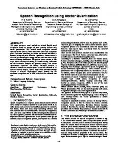
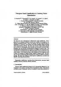
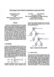
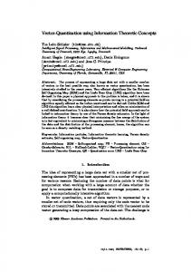
We applied our learning method for pixel classification of microscopic images of bronchial tumors [2]. The training and testing set Sa and St are built from four ground-thruth microscopic color images (RGB, 574*752 pixels). For each image, a manual segmentation is made by an expert: background (class 1), cytoplasm (class 2), nucleus (class 3). As the number of pixels in each class is not balanced in the images (1: 89%, 2: 7%, 3: 4%), only a subset of the pixels of classes 1 and 2 was selected by random to build Sa and St , so that each class has the same number of examples (≈ 60000 by class). Three training sets Sai (testing sets Sti ) are built from the Sa (St ) in order to produce binary decision problems (method one against all [11]). For each binary problem a model θi and BDF hiθ is built with our learning method. To avoid any biais for model selection the recognition rate of a BDF hiθ is evaluated from testing set Sti . Figures 1(a) and 1(d) illustrate for each BDF hiθ with a kernel KβL (optimal value of C is searched) the evolution of the recognition rate and of the number of SVs according to the level of simplification k. That is done for all the classical color spaces retained. One can notice that improvement of RR is obtained only for small values of k. Moreover, the choice of a color space which optimizes the DFQ depends to the trade-off between complexity and recognition rate. These remarks corroborate the choices which were made in the definition of our learning method. Tables 3 illustrate results obtained with our learning method by using a kernel KβL and KβG . Table 2 gives the values of configuration cp cp 2 κi 1 constants for all the configurations used. The A 0.0001 0.01 1 column κi represents two cases: the first one B 0.01 0.01 1 is a microship transformation (κi = 1) and C 0.03 0.03 1 the second one is a software transformation D 0.01 0.01 T i/T (κi = Ti /T with Ti the time P to compute the Table 2: values of constants color component i and T = i∈[1,...,nE ] Ti ). In tables 3 HCS indicates hybrid color spaces used by the BDF, ∆t the training time, and in column DF is mentioned after θ the configuration which is used. These results show that our learning method produces BDF with reduced complexity and efficient in generalization. The choice of a specific hybrid color space for each BDF generally improves the recognition rate. The improvement with the use of kernel KβL is very significant (≈ 5%) with h2θ . For this problem, the choice to use a kernel KβG in comparison with KβL does not improve the recog2 nitionP but increases the BDF complexity. Indeed, h(x) = dβ (x∗ , x) + b∗ with x∗ = i∈SV αi∗ yi xi when kernel KβL is used, then the number of SVs does not penalize the BDF complexity. However, although it seems logical to choose zero or very low values for cp1 , results (Tab. 3: left, configuration A and B) show a significant increase in time for the selection of a model without significant improvement of the recognition rate. Those results (Tab. 3: configuration B and D) also show that the uses of κi constants allow to select a hybrid color space according to its cost. In particular, in the case of software implementation the
R, G, B components are mostly used and those requiring a nonlinear transformation lesser used, but the recognition rate still is as efficient. As actually the whole process of microscopic images segmentation is software performed, then we have used the BDFs produced with the configuration D and a kernel KβL .
1000
97%
96%
94%
93%
RGB XYZ LAB LUV LCH YCH1CH2 I1I2I3 HSL YCBCR
92%
91%
Number of SV
Recognition Rate
95%
100
RGB XYZ LAB LUV LCH YCH1CH2 I1I2I3 HSL YCBCR
10
1
90% 0
1
2
3
4
5
6
7
8
0
9
1
2
3
4
5
6
7
8
9
k
k
(a) h1θ : RR .
(b) h1θ : nSV . 1000
81% 80%
100
78% 77% 76%
RGB XYZ LAB LUV LCH YCH1CH2 I1I2I3 HSL YCBCR
75% 74% 73%
Number of SV
Recognition Rate
79%
RGB XYZ LAB LUV LCH YCH1CH2 I1I2I3 HSL YCBCR
10
1
72% 0
1
2
3
4
5
6
7
8
9
0
1
2
3
4
(d)
h2θ :
(c)
h2θ :
RR .
5
6
7
8
9
k
k
nSV .
Fig. 1. Recognition rate and number of SVs in function of simplification level
9
Conclusions
A new learning method is proposed to build SVM binary decision functions which are efficient for pixel classification. This learning method produces BDF whose advantages for pixel classification problems are threefold: high generalization ability, low complexities and definition of a adapted hybrid color space. Future works will have to test this method on other pixel classification problems. It will also have to check the influence of several combination schemes of BDF, especially when the number of classes is higher. Later, it will also have to quantify the influence of other simplification methods and to compare other metaheuristics for model selection.
DF RR nSV HCS k ∆t h1θ,A 96.44% 2 ZCr 2 144 DF RR nSV HCS k ∆t h2θ,A 85.99% 48 Bb∗ L2 H1 CH2 SCb 5 26574 1 h 96.08% 5 RH1 3 865 h3θ,A 90.48% 63 Y1 L∗ a∗ u∗ 6 29540 θ,B 2 ∗ h 85.90% 10 RXa H Y 1 2 Y3 3 1239 θ,B h1θ,B 96.50% 2 Cr 2 140 3 ∗ ∗ h 90.43% 4 BY u v 2 708 θ,B h2θ,B 84.98% 18 L∗ b∗ u∗ CI2 S 4 2352 1 h 95.66% 2 R 1 482 h3θ,B 89.79% 2 Gu∗ Cb 1 147 θ,C 2 h 85.17% 10 RH Y Y 1 2 3 3 1223 θ,C h1θ,C 96.50% 2 Cr 2 140 3 ∗ h 89.47% 2 b 0 434 θ,C h2θ,C 82.82% 3 SCr 1 179 1 h 95.66% 2 R 1 440 h3θ,C 89.73% 2 v ∗ 1 140 θ,D 2 h 85.78% 10 RY Ch Y C 3 1174 1 1 3 r θ,D h1θ,D 95.66% 2 R 2 151 3 hθ,D 90.45% 5 GB 2 409 2 ∗ hθ,D 83.53% 2 RBb SL2 Cr 2 397 h3θ,D 90.09% 4 GB 2 197 Table 3. Results with a microscopic image pixels set by using a kernel KβL (left) or a kernel KβG (right)
References 1. Vandenbroucke, N., Macaire, L., Postaire, J.G.: Color image segmentation by pixel classification in an adapted hybrid color space: application to soccer image analysis. Comput. Vis. Image Underst. 90 (2003) 190–216 2. Meurie, C., Lebrun, G., Lezoray, O., Elmoataz, A.: A comparison of supervised pixels-based color image segmentation methods. application in cancerology. In: WSEAS Transactions on Computers. Volume 2. (2003) 739–744 3. Vapnik, V.N.: Statistical Learning Theory. Wiley edn. New York (1998) 4. Platt, J.: Fast training of support vector machines using sequential minimal optimization, advances in kernel methods-support vector learning, MIT Press (1999) 185–208 5. Lebrun, G., Charrier, C., Cardot, H.: SVM training time reduction using vector quantization. In: ICPR. Volume 1. (2004) 160–163 6. Gersho, A., Gray, R.M.: Vector Quantization and Signal Compression. Kluwer Academic (1991) 7. Kudo, M., Sklansky, J.: Comparison of algorithms that select features for pattern classifiers. In: Pattern Recognition. Volume 33. (2000) 25–41 8. Hao, J.K., Galinier, P., Habib, M.: M´etaheuristiques pour l’optimisation combinatoire et l’affectation sous contraintes. In: Revue d’Intelligence Artificielle. Volume 13. (1999) 283–324 9. Chang, C.C., Lin, C.J.: LIBSVM: a library for support vector machines. Sofware Available at http://www.csie.ntu.edu.tw/˜cjlin/libsvm (2001) 10. Collobert, R., Bengio, S.: SVMTorch: Support vector machines for large-scale regression problems. In: Journal of Machine Learning Research. Volume 1. (2001) 143–160 11. Hsu, C.W., Lin, C.J.: A comparison of methods for multiclass support vector machines. In: IEEE Transactions in Neural Networks. Volume 13. (2002) 415–425 12. Glover, F., Laguna, M.: Tabu search. Kluwer Academic Publishers, Boston MA (1997)