Fast range image segmentation by an edge detection ... - CiteSeerX

Fast Range Image Segmentation by an Edge Detection Strategy Angel D. Sappa

Michel Devy LAAS-CNRS 7, Avenue du Colonel Roche 31077 Toulouse, Cedex 4, France sappa @ ieee.org michel@ laas.f r

Abstract

by compact representations. Then, subsequent processing can be done within this new geometric domain instead of with individual data points contained in the given range image. Segmenting the given range image into a set of surfaces and then representing these surfaces by some compact geometrical primitives is one of the typical way to obtain higher level representations.

This paper presents an edge-based segmentation technique that allows to process quickly very large range images. The proposed technique consists of two stages. First, a binary edge map is generated; then, a contour detection strategy is responsible for the extraction of the dizerent boundaries. The jirst stage generates a binary edge map based on a scan line approximation technique. There is a difference with the previous techniques, as only two orthogonal scan line direction are considered. The planar curves defined by the elements contained in each scan line are approximated by oriented quadratic curves. The representative points from each curve are used to define a binary edge map. The second stage is a new approach to the classical contour extraction problem. It shows a difference with the previous approaches which use the enclosed surface information: with the suggested technique, boundaries are obtained by using only the information contained in the binary edge map. It consists in linking the edge points by applying a graph strategy. Experimental results with large panoramic range images are presented.

Range image segmentation traditionally relied on [ 1 ] [ 21 [31. Region-based region-based techniques approaches consist in grouping points into connected regions according to some similarity criteria. Although these techniques bring acceptable results, they have as a common problem the definition of the initial seed regions and the determination of the number of clusters. In order to tackle these problems [ l ] presents a robust clustering algorithm which can be used for range image segmentation. Other authors solve the previous problems by means of hybrid techniques (edge-based segmentation and region-based segmentation) [4][5][6]. Through these hybrid techniques, the information provided by edge detection stage is used to estimate the number of regions necessary to initialize the clustering algorithm. In these cases, the edge detection techniques are carried out only to guide and improve the clustering techniques applied to the region-based algorithm. Techniques such as those mentioned above involve high CPU time. It is not really an issue when small range images are considered; however, when very large range images have to be processed, the high CPU time prohibits the use of this kind of algorithm. For example, [7] presents a segmentation algorithm that requires a few hours to extract regions from a range image defined by 480x640 points. But when a panoramic range image defined by 1400x8000 points has to be processed, the CPU time makes it difficult to use. '

1. Introduction Range images are gaining popularity in different fields since they permit the efficient acquisition and representation of 3D information. Thus, range sensor are evolving continuously, allowing nowadays to digitalize a full scene with high resolution in a short time. The algorithms and the techniques developed to process range images have also to evolve with the same dynamism to enforce the processing of whole information rapidly. In order to accelerate further processing, dense range images have to be represented at a higher abstraction level

On the contrary, few segmentation works are based on edge-based techniques only. Edge-based approaches consist firstly in locating the points lying on edges, then, linking them to obtain the contour that defines each region. The main problem of these techniques is that they

This work has been carried out as part of the CAMERA project (CAd Modelling of Built Environments from Range Analysis). CAMERA is an EC funded TMR network (ERB FMRX-CT97-0127)

292

0-7695-0984-3/01 $10.00 0 2001 IEEE

Processing Column: n Original Range Image

" .I I

Rows +

I

Processing Row: m

-7-------I

I

I

n

*

Columns

Noisy Data Filtering Jump Edge Detection

Quadratic Approximation

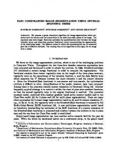
Figure 1. Illustration of the steps required to generate a binary edge map. cannot guarantee closed boundaries, because some edge points are not correctly detected. In spite of that, edgebased approaches seem to be the most attractive option when a large range image has to be processed. This paper presents an edge-based segmentation algorithm based on scan line processing. It consists of two stages. First, a binary edge map is generated by means of a scan line approximation technique. Then, the points of that map are linked, generating the boundaries that enclose each region. The works is organized as follows. Section 2 presents the technique used to generate a binary edge map. The contour extraction strategy is presented in Section 3. Section 4 shows experimental results through panoramic range images. Finally, conclusions and further improvements are given in section 5.

obtained by analyzing two orthogonal directions. Thus defining rows and columns as scan lines is enough. This first stage consists of two steps. First, the data points defining the scan lines (rows and columns) are filtered and the jump edges are detected. Second, each scan line is approximated by oriented quadratic curves. From those curves the representative points are extracted generating the binary edge map representation. Fig. 1 illustrates both steps, they are described below.

2.1. Noisy data filtering and jump edge detection A scan line is a profile digitalization which can be represented by a planar curve. By analysing that curve it is possible to detect crease edges, jump edges and noisy data. Crease edges are those points where a discontinuity in the surface orientation appears. Jump edges are defined by a discontinuity on the surface, while noisy points are defined by a surface and orientation discontinuity. In the current implementation, instead of assuming that the recursive algorithm which approximates each scan line will detect the noisy data-as was considered in [lo]-a local filtering algorithm has been implemented. It consists in linking consecutive points along a scan line and computing the distance of each segment defining that polyline. The segments with a length higher than a given threshold are the ones selected. The threshold value is obtained by considering a uniform digitalization of the surface. Next, from each of those segments mentioned above, the orientation of its normal vector is used to determine

2. Binary edge map generation This section describes the technique proposed to generate a binary edge map. It consists in approximating each scan line by means of a set of quadratic polynomial functions. Previous works dealing with scan line approximation were presented by [4][8][9]. In [9], each scan line is approximated by means of a set of straight line segments; only the points contained in the rows are used to define each scan line. On the contrary [4] and [SI approximate the scan line by using quadratic functions. In both works, rows, columns and diagonals are considered as scan lines. Compared to the previous proposals, the current work considers rows and columns as scan line; but not diagonal. Every edge contained in a range image can be

293

Pf(x,r)’ P m ( x , y ) * Pl!x.,y) are the first, middle and last points. Then, before obtaining the parameters of function ( I ) , the points of the polyline are rotated around the first point until the configuration:

’

PI(?.) = PI(?) P n w

(2)

whether the points defining that segment are noisy points or not, or to determine if that segment corresponds to a jump edge. Given an edge BC which has a length higher than a threshold o, the algorithm proceeds by computing the a n g l e s 3 between the normal vector associated with segment BC, N E , and each of the normal vectors N j associated with its consecutive edges. Fig. 2 illustrates the possible cases. In the case of crease edge, these long segments are preserved. They represent a surface with an orientation similar to the sensor viewing direction. In the case of jump edge, the segment is removed, thus cutting the polyline it defines. Points B and C are retained. During the next step, they will be used by the quadratic curve approximation algorithm, respectively as last and first points. Finally, in the noisy data case, the noisy point B is removedwith both segments defined by it. A new segment AC is obtained, linking the previous and the following point; this segment is considered as part of the polyline. This scan line filtering process removes the noisy data and cuts the original scan line into a set of polylines, according to the jump edges of that curve. Each one of these polylines is approximated by oriented quadratic functions. The approximation step will be described in the following section.

is reached. Next, the parameters of function (1) are obtained. The approximation error between the obtained quadratic function and every point of the rotated polyline is computed. If this error is greater than a given threshold 6, the polyline is split into two polylines at that point where the biggest error appears. That point is then considered as last point, the middle point is computed, the points of that polyline are rotated according to (2), and the parameters of (1) are computed again. This splitting algorithm is applied recursively while the approximation error is greater than 4 . The result of this recursive algorithm is a set of quadratic curves approximating the given polyline. Once this polyline is approximated, the recursive algorithm is carried out over the next polyline of the given scan line. From each quadratic curve, the first and last pointsthose used to compute the parameters of function (1)are selected and their positions on a binary map are labelled. The original range image can be provided by any 3D sensor, like stereovision or laser range finder. In this way, the binary edge map can be represented as a two dimensional array S, where each element S(r,c) is a binary value indicating whether or not the point has been selected by the previous approximation technique. 3D coordinates P(x, y, z ) are associated to each selected point on the binary map. Once all the polylines of a given scan line have been approximated, the algorithm starts again from the filtering step (Section 2.1.) over the next new scan line. If, on the and columns-have been contrary, all scan lines-rows processed, the obtained binary edge map is the final result and the next stage is applied. Fig. 3 shows the binary edge map after processing a panoramic range image.

2.2. Scan line approximation

3. Contour extraction strategy

D

C D

Figure 2. Examples of: (leff) crease edge; (middle) jump edge; (right) noisy data and jump edge.

At this step, a scan line has been cut into a set of polylines. The next algorithm is applied to every polyline separately and consists in approximating each one of them by a set of quadratic functions oriented along edge y:

y = ax2+bx+c

The contour extraction is a common problem within the image processing field. However, so far it did not get so much attention. Most of the authors preferred to develop solutions for their specific problems. For example, [5] presents an edge linking algorithm to close a one pixel gap in any one of the four directions. Some other works tackle the contour extraction problem by analysing the enclosed surfaces [4][11]; simultaneously, contour and region are extracted. [ l 11 deals with the understanding of natural scene from range

(1)

The approximating step has been implemented by means of a splitting algorithm. The quadratic function is obtained by using the first, middle and last point of the considered polyline. It will be supposed that

294

Figure 3. (fop) Binary edge map obtained from a panoramic range image defined by 74OOx8OOO points; for scale reasons some neighbouring edges seem to be a thin surface instead of a pair of edges. (bottom) Enlargements of different regions. cess is restricted to one direction. This direction-guided dilation is applied only over the ending points of the contours. The direction of dilation is determined from the last three points connected with the ending point. Thus, from these four points, one gets an average direction which will be considered as the direction of dilation. Since some uncertainty still remains about the direction vector, i t is suggested to include surrounding points to that direction. Instead of being carried out along a single straight line, the dilation is applied along a conic region; the apex of that cone is the ending point of the open contour. This approach can deal with thin regions. Sometimes, however, considering the last three segments of an open contour only-the last point plus three previous ones over that contour-cannot be enough to obtain the good boundary direction. Normally, this technique cannot handle most of

images; in the area close to the ending point of an edge, a local analysis of the depth is performed in order to select an optimal edge dilation direction. Jiang and Bunke [8] brought forward an adaptive approach that extracts closed contour by applying a process of hypotheses generation and verijication. This algorithm is based on the consideration that any contour gap can be closed by dilating the input edge map. Thus, a single dilation operation followed by a region verification is applied until all regions are labelled. The problem is that, as the dilation is performed in all directions, thin regions are liable to disappear, due to the fusion of the contours enclosing them. An extension of the previous approach is presented in [12]. There, the geometry of contours is taken into account in order to apply the dilation-the dilation pro-

295

the possible pathological cases emerging when real range images are processed. Those problems may appear when the final points are affected by noisy data or when the open contours describe curved shapes; in this last case, the direction vector used for the dilation is not representative of the boundary direction. Most of the aforementioned techniques are based on the consideration that boundaries can be extracted by dilating the input edge map and that any contour gap will be closed. It may be good to deal with the typical open contour but the common issue of these techniques is to find the good dilation direction in a general way. On the contrary, this work links the points from the binary edge map by applying a graph representation and by using the graph theory. This section presents the technique used to obtain contours. It consists of three stages. Firstly, the points from the input binary edge map are triangulated over its 2D space. Then, a weighted graph is generated, with the points of that triangular mesh as nodes and the edges of the triangles as links. A weight (or cost) is associated to each edge of this graph. It corresponds to the 3D distance between the two points joined by this edge. Secondly, the minimum spanning tree (MST) is computed from the weighted graph. Thirdly, a filtering stage removes all short branches generated by the MST algorithm. These stages are described below.

Figure 4. Section of the 2D triangular mesh obtained from the binary edge map triangulation. some are missed by the edge detection algorithm, one can assume that one or two points could be missed. As far as these cases are concerned, and through the current implementation, we set 3 f i units as 2D threshold distance. This value corresponds to the case where two consecutive points are missed along a diagonal. After removing all those edges with a length higher than the previous value, the threshold filter is applied to the remaining edges, but this time considering their 3D length. Because the triangulation algorithm has been carried out over a 2D space, points which are neighbours in that space (2D projection), may be placed at different sides of a jump edge. This second stage of the filtering algorithm has been developed to remove this kind of edges, thus reducing further MST computing time. The 3D value used as threshold is set according to the jump edge value associated with the given range image.

3.1. 2D triangulation and graph generation This first step consists in triangulating the points from the binary edge map obtained in Section 2 through a 2D Delaunay algorithm. The point positions ( 4 c ) in the array S are considered in that 2D space through the triangulation algorithm. The cost to perform the 2D Delaunay triangulation is O(nlogn), with n being the number of points. Fig. 4 shows a section of the planar triangular mesh found after triangulating the given binary edge map. Small triangles are generated by points that define the same boundary, and big isosceles triangles are too, but by points from different boundaries. Now, the previous triangular mesh is considered as a weighted graph G: the vertices of the triangular mesh are the nodes of that graph and the edges defining the triangles are its edges. Each edge of the graph has associated a cost which is defined by the 3D distance between the points joined by this edge. Because only boundaries must be extracted from this graph, edges with a cost higher than a given threshold are removed. This threshold jilter is applied taking into account, first, a 2D distance and then a 3D distance. The threshold for the 2D distance is defined considering that the surface is regularly sampled. So, points belonging to the same boundary turn out to be neighbours in the binary map. However, knowing that some points are noisy or

3.2. Minimum spanning tree generation The aim at this stage is to obtain the shortest path linking all the edge points. This is achieved by computing the minimum spanning tree of the previous weighted graph. Given a weighted graph G, the MST of G is the acyclic subgraph of G that contains all the nodes and such that the sum of the costs associated with its edges is minimum. The MST of a graph with m edges and n vertices can be efficiently computed in O(mlogn) by applying Kruskal’s algorithm [13]. In the current implementation, due to the previous threshold filter, each point can be considered as having a maximum of k connections; then the cost can be bounded by 0 ((W2)nlogn). Fig. 7(top) shows an example of the MST resulting from the filtered triangular mesh (Section 3.1), an enlargement is given in Fig. 5 . The resulting tree is a set of unconnected branches; It is due to the threshold filter which removed connections between them. Thus, the algorithm used to built the MST does not succeed in generating a single tree. As expected, the generated trees go along the edge points, defining the future boundaries by

296

Opening Algorithm

%

Original Tree Dilation

_ - -*---.-.-

'

---. Figure 5. Enlargement of the resulting minimum spanning tree. linking them. Moreover, the algorithm generates several short branches which are removed during the following stage.

igure 6. Illustration of the opening algorithm.

3.3. MST filtering by an opening algorithm The resulting MST can be understood as a set of independent trees. Each of them is a polyline whose segments are the graph edges. As shown in Fig. 5 , several short branches-isolated or linked with the main path-were generated from the MST. The first set belongs to isolated noisy data which have been linked by the MST; the second one belongs to information redundancy in some crease or jump edge regions. Thus, the minimum spanning tree from the weighted graph is not enough to define the boundary of the regions. Before, it is necessary to remove those short branches (see enlargement shown in Fig. 5). In order to perform the removal process, a kind of opening algorithm has been implemented. This algorithm consists in performing an iterative erosion process followed by a dilution stage applied as many times as the erosion requires. The opening algorithm considers the segments of the polyline-i.e. edges from the graph-as basic processing elements (like pixels in an intensity image). Those segments linked from called end segonly one of their ending points-so ments-are removed during the erosion stage. This stage is applied t times and at each iteration, all the end segments of that configuration are removed. The number of iterations depends on the input binary edge map. Through the examples chosen, ten erosion iterations were applied to remove the short branches. Once the erosion process is completed, a dilation process is performed. This algorithm is carried out over the end segments left by the erosion process. It consists in putting back the segments connected with each one of the end segments present at each iteration. The number of dilations is the same as the number of erosions. Thus in

order to execute the dilation process, it is necessary to store the history of those end segments left by the erosion process. Fig. 6 shows an illustration of the proposed opening algorithm. Fig. 7(middle) shows the resulting boundaries obtained from the opening algorithm application. Enlargements of different regions are given in Fig. 7( bottom). Finally, after removing the single branches, the different boundaries are extracted and labelled.

4. Experimental results The proposed algorithm has been tested with different panoramic range images. CPU times have been measured on a Sun Ultra 5 . The example used through this paper corresponds to a 1400x8000 (rows x columns) panoramic range image. Fig. 3 shows the binary edge map obtained from the technique proposed in Section 2; it contains 400,419 points; the CPU time necessary to get that map was 2,473.78 sec. From that binary map, a 2D triangular mesh with 782,039 triangles was created. The 2D Delaunay triangulation was computed in 138 sec. Then, a graph with 622,825 edges was obtained by removing long edges by means of the threshold filtering stage. From that graph the MST was generated. Fig. 7(top) shows the obtained result composed of 353,257 edges. The CPU time to compute it was 415.28 sec. Fig. 7(middle) and (bottom) shows the boundaries resulting from the opening process. This opening algorithm took 104.94 sec. The boundary representation is composed of 144,005 edges. The number of opening iterations is a parameter defined by the user; the aim is to remove all those branches generated by

297

.

I

Figure 7. (top) Resulting MST, several unconnected branches have been generated from noisy data. (middle) Boundaries obtained after filtering (opening process) the MST showed above. (bottom) Enlargement of different regions.

since some real edges will be taken away. On the other hand, only a few iterations will produce bad results too, as only short branches will be removed. In the current implementation, ten iterations, erosion and dilation, were used.

rithm took 149.33 sec. After removing long edges, a graph with 739,082 edges was created. From that graph the MST was obtained in 582.45 sec. containing 413,714 edges. Finally, the opening algorithm extracted the contours in 89.47 sec. This final representation (Fig. 8) contains 213,188 edges.

Fig. 8 shows another example of the contours extracted by means of the proposed technique. The binary edge map obtained from the original range image was computed in 2,234.42 sec.; it contains 464,695 points. The 2D triangular mesh generated by those points is composed of 910,592 triangles. The 2D Delaunay triangulation algo-

Other panoramic range images from the CAMERA project and some range images from industrial environments were tested by the technique presented in this paper -for space limitations they do not appear in this paper; however, they can be viewed on the web page of the authors.

the noisy points of the binary edge map. On the one hand,

a high number of iterations does not lead to a good result

298

Figure 8. Contours extracted from a panoramic range image defined by 7400x8000 points. E. Natonek, Fast Range Image Segmentation for Servicing Robots, IEEE Int. Conf. on Robotics and Automation, Leuven, Belgium, May 1998,624-629. M. A. Garcia and L. BasaAez, Fast Extraction of Surface Primitives from Range Images, 13th IAPR Int. Conf. on Pattem Recognition, vol. 111, pp. 568-572, Vienna, Austria, August 1996. 0. Pereira Bellon, A. Direne and L. Silva, Edge Detection to Guide Range Image Segmentation by Clustering Techniques, IEEE Int. Conf. on Image Processing, Kobe, Japan, October 1999. E. AI-Hujazi and A. Sood, Range Image Segmentation with Applications to Robot Bin-Picking Using Vacuum Gripper, IEEE Trans. on SMC, Vol. 20, No. 6, pp. 1313.1325, December 1990. K. Koster and M. Spann, MIR: A n Approach to Robust Clustering-Applicationto Range Image Segmentation, IEEE Trans. on Pattem Analysis and Machine Intelligence, Vol. 22, No. 5, pp. 430-444, May 2000. P. Besl and R. lain, Segmentation Through Variable-Order Surface Fitting, IEEE Trans. on Pattern Analysis and Machine Intelligence, Vol. 10, No. 2, pp. 167-192, 1988 X. Jiang and H. Bunke, Range Image Segmentation: Adaptive Grouping of Edges into Regions, Computer Vision-ACCV’98(R. Chin and T. Pong, Eds.), pp. 299-306, Springer-Verlag,Berlinmew York, 1998. X. Jiang and H. Bunke, Fast Segmentation of Range Images into Planar Regions by Scan Line Grouping, Machine Vision and Applications, Vol. 7, No. 2, pp. 115-122, 1994. [IO] X. Jiang and H. Bunke, Edge Detection in Range Images Based on Scan Line Approximation, Computer Vision and Image Understanding, Vol. 73, No. 2, pp. 183-199,February 1999. II ] S. BetgC-Brezetz, R. Chatila and M. Devy, Natural Scene Understanding for Mobile Robot Navigation, IEEE Int. Conf. on Robotics and Automation, San Diego, USA, May 1994,730-736. 121 X Jiang, An Adaptive Contour Closure Algorithm and Its Experimental Evaluation, to appear at IEEE Trans. on Pattem Analysis and Machine Intelligence. [ 131 K. Rosen, Discrete Mathematics and its Applications. McGraw-Hill, Inc., New York, second edition, 1990. [I41 A. Hoover et al., An Experimental Comparison of Range Image Segmentation Algorithms, IEEE Trans. on Pattern Analysis and Machine Intelligence, Vol. 18, No. 7, pp. 673689, July 1996

5. Conclusions and further improvements This paper presents a fast technique to deal with large range image segmentation based on an edge detection approach. Only the information about the edges is used; none assumptions about the parameters of the enclosed surfaces have to be made. This technique consists of two stages. Firstly, a binary edge map is generated by analysing the scan line profile. Two orthogonal scan line directions are taken into account. Each one of them is approximated by quadratic planar curves. From these quadratic approximations, the first and last points are considered in order to define the binary map. Secondly, the points of the binary map are used to define a graph. Next, the MST of that graph is obtained. Finally, an opening algorithm removes short branches from that tree and the different contours are extracted. The current technique only uses the edge information. A further work will try to improve the segmentation result by means of some additional post-processing by considering some surface information. Thus, by using the parameters of the enclosed surfaces, neighbouring regions can be merged according to some similarity criteria. Moreover, some edges which have been removed during the opening stage, can be recovered by studying the surface property. An additional work will deal with the automatic determination of the number of opening iterations, according to the noisy data. The technique developed in [ 141 will be used to make a comparison with the previous approaches. The proposed technique was developed to handle large range images; therefore, these ones are necessary to make some comparisons. However, most of the time it is impractical to use some regionbased segmentation techniques, like the one presented in [7],when large range images are considered.

6. References [I] H. Frigui and R. Krishnapuram, A Robust Competitive Clustering Algorithm with Applications in Computer Vision, IEEE Trans. on Pattem Analysis and Machine Intelligence, Vol. 21, no. 5, pp. 450-465, May 1999.

299