Range Image Segmentation by Surface Extraction

Range Image Segmentation by Surface Extraction Using Improved Robust Estimator and Genetic Algorithm Paulo F. U. Gotardo1 , Olga R. P. Bellon1 , Luciano Silva2 , and Kim L. Boyer3

1 Departamento de Inform´atica Universidade Federal do Paran´a, Curitiba (PR), Brasil {paulo,olga}@inf.ufpr.br

2 Prog. de P´os-Gradua¸c˜ao em Eng. El´etrica e Inform´atica Industrial Centro Federal de Educa¸c˜ao Tecnol´ogica do Paran´a, Curitiba (PR), Brasil [email protected]

3 Department of Electrical Engineering The Ohio State University, Columbus (OH), USA [email protected]

Abstract This paper presents a novel image segmentation method employing an improved robust estimator to iteratively detect and extract distinct surfaces from range images. Our robust estimator is based on MSAC and RANSAC algorithms and is designed to eliminate the extraction of false surface components and, thus, to avoid over-segmentation.

It also

employs a genetic algorithm specifically designed to better accelerate the optimization process of surface extraction, while avoiding premature convergence. Our approach lends itself naturally to parallel implementation and application in real-time tasks. The method fits well into several of today’s applications such as target detection and autonomous navigation, for which obstacle detection on a ground plane, but not description or reconstruction, is required. The segmentation algorithm was applied to a number of range image databases and competes favorably against other eleven segmenters using the most popular evaluation framework for planar surfaces. Our segmenter is not limited to planes and is being extended to extract higher order curved surfaces and to segment more complex objects.

1

Introduction

To perform tasks such as object recognition, autonomous navigation, industrial inspection, or reverse engineering, computer vision systems must be able to identify real world objects reliably from sensed environmental data in the form of digital images. Since the image interpretation task is often very complex, an intermediate segmentation process is needed to partition the data, yielding a few higher-level structures (usually surfaces) which are analyzed and related to each other to identify the objects in the scene. Thus, a fundamental requirement for a computer vision system to obtain a reliable object representation is an accurate segmentation process that preserves object shapes and edge locations. However, image segmentation is one of the main challenges in computer vision. Processing digital images to segment a number of objects – possibly in different positions 2

and with different sizes and shapes – is still a difficult task. It depends on correct feature extraction from images that may be corrupted by noise and other sensor errors. Many of the segmentation techniques reported in the literature [1]–[19] work on range images [20], which contain explicit 3D information on the scene geometry. Techniques for range image segmentation usually employ one of two main approaches: (1) region-based segmentation [3, 5, 6, 7, 12, 13, 15, 16, 17]; or (2) edge-based segmentation [2, 10, 18]. Since, whatever the chosen approach, the segmented image will contain both region and edge information, some hybrid segmentation techniques have also been developed combining these two complementary approaches [1, 4, 11, 14, 19]. As demonstrated by Hoover et al. in the evaluation of four state-of-the-art range image segmentation algorithms [8], and as restated later by Jiang et al. [9], the segmentation problem is still not solved even for simple scenes containing only polyhedral objects. The segmentation comparison framework developed by Hoover et al. has been widely adopted for evaluating segmentation algorithms [9, 10, 14, 15, 16]. It also served as the basis for the development of other comparison frameworks, such as for evaluating curved surface range image segmenters [21]. Computer vision systems are often applied in man-made environments, in which objects or object parts are described by simple geometric primitives such as straight lines, planes, and other low-level curves and surfaces [22, 23, 24]. Therefore, reliable characterization and extraction of these image elements are of fundamental importance in image understanding. An often adopted approach to the geometric characterization of surfaces in range images is to fit surface models to range data subsets and then calculate geometric features, such as surface orientation and curvature, using the estimated surface parameters [25]. One problem that arises from this fitting approach is that even if the surface model (e.g. plane, quadric) is known a priori, the parameter estimation process may be corrupted by image noise. Another problem is that least squares estimate [26], although optimal for Gaussian perturbations, is very sensitive to other classes of noise because all data points are taken into account equally 3

and one arbitrarily bad point, an outlier, can completely corrupt the fit, regardless of the number of good points. Outliers may be either noisy points, or points from a different surface. Thus, to obtain a reliable surface segmentation the estimation process must avoid the unwanted effect introduced by outliers. Statistical techniques known as robust estimators [27, 28, 29, 30] have become very popular in computer vision because they are able to tolerate data from different statistical populations (e.g. neighboring surfaces, impulsive noise) while estimating the parameters of the dominant population (surface). Some of these techniques [17, 31, 32] can tolerate more than 50% outliers without corrupting the fit. Besides locally fitting surface models to a set of points, these robust estimators make it feasible to solve the more complex problem of extracting whole surfaces – i.e. identifying not only the surfaces parameters but also the sets of points (inliers) that actually describe them [11]. Geometric primitive extraction plays an important role in model-based computer vision because these primitives may be used to describe and identify objects or object parts. Roth and Levine [11] show that geometric primitive extraction is essentially an optimization problem whose objective is to find the geometric primitive hypothesis minimizing a robust cost function, which may exhibit many local minima. Therefore, it is potentially a timeconsuming task and must be performed with as few cost function evaluations as possible. Because of this, the random sampling technique, initially employed to generate a minimal set of points required to instantiate a primitive hypothesis, has been replaced in some extraction methods [12, 17, 33] by more efficient genetic algorithms [34]. Generally, segmentation algorithms employing robust estimators for surface extraction [3, 11, 12, 13] process the whole image to extract its surfaces sequentially. In each iteration, the inliers of the extracted surface are removed and, if the number of remaining points is sufficiently large, a new iteration is started. According to this extraction model, it is possible to extract geometric primitives described by less than 50% of the data set. However, one problem of this procedure is that if the inliers 4

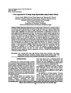
(a) Range image

(b) Ground truth regions

(c) Inliers for region 1

(d) Our estimator’s inliers for region 1

Figure 1: Extraction of false surface component and over-segmentation caused by pseudoinliers, which should be classified as outliers and discarded.

do not yield a connected region (e.g. due to image noise), over-segmentation may occur. Another drawback is that some false surface components may be extracted. The reason is that the true extent of the imaged surfaces are not always known and, therefore, some points of neighboring surfaces, which are intercepted by an unbounded surface (model instance) being extracted, may be incorrectly identified as (pseudo-) inliers. Also, the intercepted surfaces may be split into two or more pieces. This is illustrated in Figs. 1(a)–1(c), where region 2 is intercepted by pseudo-inliers of an unbounded planar surface estimated for region 1. In this case, one needs to correctly classify pseudo-inliers as outliers to discard them and avoid over-segmentation of region 2 (Fig. 1(d)). To accelerate the extraction process, one approach is to reduce the computational expense of the robust cost function evaluation by using an initial, rough edge-based segmentation to partition the search space from which surfaces will be extracted. However, the computed edge map is usually neither complete nor closed, and does little to solve the pseudo-inlier problem. Furthermore, if the detected edges are not precisely located, the extracted surfaces may be incorrectly shaped. As already mentioned, another way of accelerating the extraction process is to reduce the number of cost function evaluations required in the optimization. This is usually done by replacing the random search technique by genetics algorithms (GAs). GAs are computational 5

models of natural evolution in which stronger individuals are likely to be the winners in a competitive environment [34]. Besides presenting an intrinsic parallelism, GAs are simple and efficient techniques for optimization and search. The general principle underlying GAs is to maintain a population of possible solutions (individuals), encoded in the form of a chromosome (a string of genes), and to submit this population to an evolutionary process until some criteria can be satisfied. In this process, each individual is assigned a fitness value provided by a user-defined fitness function and the fittest individuals have more opportunities to be selected for reproduction. With the intent of creating better individuals, the crossover operation exchanges the genes of each couple of chromosomes selected for reproduction. The resulting (child) chromosomes, before being introduced to the population, may undergo mutation, a random perturbation, to enrich the genetic content of the population. Mutation occurs with a very small probability to ensure that the evolutionary process does not degenerate to a purely random search. Finally, the fittest chromosome is taken as the final solution. A drawback of GAs is the difficulty in setting their many parameters, which are problem-bound and must be empirically and carefully determined to avoid premature convergence.

In Section 2, we present a new range image segmentation algorithm [1] combining edge and region-based segmentation techniques and applying a robust estimator to extract planar surfaces from range images. This robust estimator is an improved version of the MSAC estimator [32] – which is, in turn, an improvement to the RANSAC estimator [31] – and was specifically designed to avoid the interference of pseudo-inliers in the segmentation process (Fig. 1(d)). We also have developed a new set of GA parameters to accelerate the optimization process while avoiding premature convergence. The experimental results are presented in Section 3. We evaluate our algorithm using the framework of Hoover et al. [8] and compare our results to other eleven range image segmentation methods in Section 4. Section 5 contains the conclusions and outlines future work. 6

2

Segmentation Algorithm

Our segmentation algorithm uses an improved robust estimator to extract planar surfaces from range images iteratively. Combining edge and region-based segmentation, it comprises two main stages, as shown in Fig. 2. The main purpose of the preprocessing stage is to estimate the surface orientation at each image point. This information is required by the robust estimator employed in the next stage, surface extraction. Once surface orientation is available, the first stage also builds an initial, rough edge-based segmentation. In the second stage, the resulting edge map is used to partition the search space from which planar surfaces will be extracted; this reduces the computational cost of the extraction process. Let SSS be the resulting Search Space Set. After the SSS is obtained, an iterative planar surface extraction process is started. In each iteration, only the points in the largest search space (region) in the SSS are taken into account; the others are left for future iterations. The robust estimator first extracts a set of inliers, yielding the largest planar surface in the current search space. These inliers serve as seeds for region growing to identify a connected region corresponding to the surface being extracted. When regions stop growing, the largest connected component is taken as the resulting region, removed from the search space, and (1) preprocessing

median filter smoothing

(2) surface extraction

range image

search space partitioning

step edge detection

robust surface fit

local planar fit

normal vectors

region growing/extraction

roof edge detection

edge map

search space update

segmented image

T

search space set empty?

F

Figure 2: The two main processing stages of the range image segmentation algorithm. 7

saved in the output segmentation image. After this, connected components remaining in the search space, and whose sizes are larger than a threshold ts (which may be a small percentage of the image size), are added to the SSS. At the end of each iteration, the processed search space is removed from the SSS and discarded. While the SSS is not empty, a new iteration is started for its largest search space.

2.1

Preprocessing

The initial edge-based segmentation results from the detection of step and roof edges [2]. First, the range image is smoothed by one pass of a 3 × 3 median filter. We detect step edges by thresholding a depth gradient image using an automatic threshold value calculated from the mean and standard deviation of the gradient values [35]. Roof edges are detected by thresholding a gradient image for the angular difference in surface orientation between neighboring pixels. Surface normal vectors are estimated at each pixel p by a local least squares planar fit. This process uses step edge information to consider only those points on the same side of a step edge and within an N × N neighborhood centered at p. To improve the estimates near roof edges, once the local fit has been performed, a small M × M mask (M < N ) is centered at p. Pixel p is then assigned the normal coefficients of that pixel presenting the lowest fit error among all pixels covered by this smaller mask. Since the combined step and roof edge map is used only as a rough, initial segmentation, edge thinning and closing are not required. Also, each connected region in this raw edge map may correspond to multiple surfaces separated by smooth edges that were not detected. In the next stage, all such regions are treated as disjoint search spaces from which a number of planar surfaces should be extracted. 8

2.2

Surface Extraction

The search space partitioning is done by identifying connected regions in the edge map. Those regions larger than a pre-specified threshold ts are considered to be search spaces and are assigned to the search space set (SSS). Then the iterative planar region extraction process begins and, at each iteration, only the largest search space (region) in the SSS is considered to undergo (1) robust surface fit, (2) region growing/extraction, and (3) search space update. Here, we describe these three procedures in detail.

2.2.1

Robust surface fit

Given a search space Si ∈ SSS, the first step of each iteration uses the improved robust estimator to identify the parameters and a set of inliers (Ii ) for the largest planar surface in Si . This optimization process employs a GA in which each chromosome (individual) represents a surface hypothesis and contains 3 points (genes) from Si , defining a plane. At the end of the evolution process, the points in the chromosome presenting the best fitness value are used to identify the set of inliers which, in turn, is used in a final least squares planar fit, yielding the estimated surface parameters. The fixed-size, initial population of the GA is created with a number of chromosomes whose genes contain randomly sampled points from Si . To maintain genetic diversity in the population during the evolution process and, thus, to avoid premature convergence, duplicated chromosomes are not allowed in the population. Additionally, the much employed proportional selection is replaced by a tournament selection, in which the chromosomes in a mating couple are defined to be the fittest ones (the winners) from couples of competing, randomly chosen chromosomes. Tournament selection presents a better performance in maintaining genetic diversity [36] because it better prevents the genes of only a few good chromosomes from dominating the whole population. Avoiding premature convergence is critical because the surface extraction process requires a value very close to the global minimum of the robust cost function to be found. 9

In each genetic operation cycle of the evolution process, a mating couple is selected and two children chromosomes are created by a uniform crossover operator, which exchanges pairs of corresponding parents genes with a probability of 0.5. Uniform crossover is also known to better promote genetic recombination (diversity) than one and two-point crossover techniques [34]. After that, each child’s gene may be mutated with a small probability, Pm . The mutation operator moves the gene’s point a number of pixels (∆m ) in one of four possible directions (north, south, east or west) and inside the search space Si . The new chromosomes are evaluated using the fitness function (described below) and are included in the population. To maintain the population size constant, its two least fitted chromosomes are then discarded. The fitness function f tn(c) of chromosome c, which is to be maximized, is defined in terms of an improved MSAC estimator cost function, f (•), which, in turn, must be minimized:

f tn(c) =

1 f (Rc , NL )

(1)

where Rc is the set of the residual (Euclidean) distances rj between each point pj ∈ Si (1 ≤ j ≤ |Si |) and the hypothetical surface (ac = (a1 , ..., am ), with m = 4 for planes) whose coefficients were instantiated from the (m − 1) points in the chromosome c; and NL is the set containing the locally estimated unit normal vectors, ~nj , at point pj (obtained in the preprocessing stage). Our cost function f (•) is defined as:

f (Rc , NL ) =

n X

ρ(rj , nj )

(2)

j=1

where ρ(•) is our new robust residual term specially designed to avoid the problem caused by pseudo-inliers, as illustrated in Fig. 1(c). Introducing orientation information into the MSAC residual term allows our robust estimator to correctly reject pseudo-inliers as outliers and avoid both the extraction of false surface components and the over-segmentation of neighboring surfaces (Fig. 1(d)). Our 10

residual term ρ(•) considers a point pj ∈ Si as an inlier only if pj can be classified, similar to [6, 7], as a point which is “compatible” with the hypothetical surface ac , in the sense that the following properties are presented: 1. pj is sufficiently close to the hypothetical surface (i.e. the residual value rj is less than a pre-specified threshold σ); 2. ~nj is within an angular threshold θ with the unit normal to ac at point pj (for planes, we have a constant unit normal ~na ). With ρ(•) defined as shown in Equation 3, each inlier contributes to f (•) a cost equal to its residual distance, while each outlier contributes a constant cost, σ. The outlier residuals are discarded and, thus, have no influence on the hypothesis evaluation. In this way, maximizing the fitness function f tn(•) is equivalent to finding the surface hypothesis which minimizes the number of outliers while also minimizing the sum of the inlier residuals.    rj ρ(rj , nj ) =   σ

if

rj < σ

and ~nj · ~na > cos(θ)

(3)

otherwise

At the end of the robust surface fitting process, a final least squares fit is performed to the inliers of the best surface hypothesis, yielding the final surface coefficients ˆ a and a new set of inliers Ii .

2.2.2

Region growing/extraction

When the process described above is applied to extract surfaces from real range images, several points on these surfaces may not be classified as inliers because of noise effects. Thus, the set of inliers Ii obtained in the previous step of our segmentation process may not yield a connected region. Because of this, after the robust surface fit step, there is still the need to identify a connected region Ri enclosing all the pixels (even those corrupted by high-level noise) corresponding to the actual scene surface. 11

fitted surfaces (âi and âj)

σc Ri

Rj

decision surface

range data

Figure 3: The decision surface criterion is applied to the ambiguous region (gray area) whose points support both the neighboring surfaces. As shown in the diagram (adapted from [7]), assigning an ambiguous point to its nearest surface would not preserve the correct edge location.

To do so, the residual (σ) and orientation (θ) thresholds used in Equation 3 – which initially are set to small values to improve the precision of the estimated surface parameters, when processing noisy data – are multiplied by a small constant C, usually 2 ≤ C ≤ 4, which is a relaxation factor to our previous constraints. The resulting threshold values (σc and θc ), together with the estimated surface parameters (ˆ a) and the inliers in Ii (taken as seed points), are used as input for a region growing process that groups neighboring points which are compatible with the estimated surface. When regions stop growing, Ri is defined as the largest connected component. Since the initially detected (roof) edges may not be precisely located, this process is allowed to grow regions beyond the current search space limits. But before Ri is saved (with the label “i”) in the output image of extracted regions, we refine the edges of Ri using a decision surface criterion [7] applied to regions of “ambiguous” points (Fig. 3). These are points also assigned to another, previously extracted region Rj (with label j < i). Each ambiguous point is then assigned to the region on the same side of the decision surface, which in the case of planes is another plane passing through the line of intersection, and bisecting the space between the planes of the two neighboring regions (for curved surfaces, the local tangent planes at each pixel may be used). 12

2.2.3

Search space update

Finally, in the last step of each iteration, Si is removed from the search space set, SSS, and the connected components in Si − Ri are identified and those whose sizes are larger than the threshold ts are added to the SSS. While the SSS is not empty, a new iteration is started for the largest search space in this set. When there are no more search spaces to be processed, the surface extraction stage finishes and the output image containing all the extracted regions is the segmentation result for the input range image.

3

Experimental Results

The developed segmentation algorithm was applied to the popular ABW and Perceptron range image databases that have been used by a number of research groups [8, 9] and are available at http://marathon.csee.usf.edu/seg-comp/SegComp.html. The values (number of pixels) for the mask dimensions N and M used in the local fit of the preprocessing stage, and the minimum search space size ts , depend mainly on the size of the input images. For the ABW and Perceptron images, with 512 × 512 pixels, we have N = 15, M = 11 and ts = 100 (which corresponds to less than 0.04% of the image size). Below, we describe the experiments on setting GA parameters and segmenting ABW and Perceptron images. We also present some remarks on applications of our algorithm.

3.1

Determination of GA parameters

The GA requires that four parameters be initially specified: the population size (ps ), the mutation probability (Pm ), the mutation offset (∆m ) in number of pixels, and the number of iterations in the evolution process (ni ). To define an appropriate set of values for these parameters and also to assess the performance of the GA in avoiding premature convergence and in accelerating the extraction process, we performed the following experiment. The entire range image in Fig. 4(a) was taken as a single search space, and the GA13

(a) Search Space

(b) Inliers for the floor

(c) Inliers for the background

Figure 4: The experiment to determine the GA parameters.

based robust estimator was used to identify the inliers of the largest planar surface. One reason for using this image is that its two largest planar surfaces have slightly different sizes. The floor occupies about 30% of the ground truth (hand-segmented) image; the background about 29%. In this way, the detection of inliers of the floor plane (Fig. 4(b)) indicates that the GA was able to converge to the global minimum of our robust cost function. If inliers were detected for the background plane (Fig. 4(c)), premature convergence (to a local minimum) would be indicated. Another reason for choosing this image is that, considering the high noise level of the Perceptron images, one can assume that the inliers for the floor and background planes are fewer than, respectively, 30% and 29% of the pixels in the image. This ratio was suitable to “stress test” the algorithm and to set parameters. Subsequently, we observed that the average inlier ratio in the extraction of each region was 91% for the ABW test set and 72% for the Perceptron test set. Inlier ratios below 30% were rare, being found in the extraction of fewer than 0.5% of the ABW test set regions and in fewer than 4% of the Perceptron test set regions. We tested more than 100 combinations of GA parameter values, with 100 tests for each combination, and found that the lowest average cost was obtained with the following configuration: ps = 70 (individuals), Pm = 0.05 (5%) and ∆m = 9 (pixels).

Also,

no significant decrease in the average cost function value was observed with either small modifications to these parameters or after the 500th iteration of the optimization process. 14

Robust estimator’s cost function value

460000

Random sampling Conventional GA Our GA

455000

450000

445000

440000

435000 100

150

200 250 300 350 Number of cost function evaluations

400

450

500

Figure 5: Minimization of the robust cost function with different optimization techniques.

So, we set ni = 430 (plus the 70 evaluations to create the initial population). The results of our modified GA were compared to the results presented, in this same experiment, by the random sampling optimization technique and by a conventional GA (employing proportional selection and mutation by random substitution).

Premature

convergence – in our experiment, the detection of the background’s inliers – was detected in 36% of the tests with the random sampling technique. The conventional GA showed 20% premature convergence, while our GA exhibited 13%. Fig. 5 shows the average evolution of the robust estimator’s minimum cost function value for these three optimization techniques. As shown in the graph, the cost function value obtained by random search after 500 iterations was reached by our GA in about half the number of iterations. Furthermore, our GA took less than 275 iterations to reach the same cost function value achieved by the conventional GA after 500 iterations. Clearly, our GA offers faster optimization with superior resistance to premature convergence. 15

3.2

Segmentation of ABW and Perceptron range images

After the GA parameters were defined, the remaining threshold values to be set were σ and θ, used to identify inliers in the robust surface fit process, and the relaxation factor C, used in the region growing process. These values were experimentally set using the ABW and Perceptron training image sets: σ = 1.4 (range unit, about 0.5% of range interval), θ = 14 (degrees) and C = 3. For visual comparison, Figs. 6 and 7 present the segmentation results of our algorithm for, respectively, one ABW and one Perceptron range image, together with the results provided by the segmenters in [8], originally referred to by the names of the universities in which they where developed.

Because of space limitations, we only present the results for these two

range images, which also appear in [8]. The segmentation results for the entire ABW and Perceptron image databases can be obtained at http://www.inf.ufpr.br/imago/seg-results. The average times to segment each ABW/Perceptron image – on a PC with a single 2 GHz Pentium IV processor, 512 MB of RAM, running Linux 2.4.18 – are shown in Table 1. This table also shows the relative and absolute processing times for preprocessing, surface extraction, and the robust surface fit, which is the procedure of highest computational cost within surface extraction.

These times can be greatly reduced through parallel

implementation, mainly for the local fits of the preprocessing stage and for the evolutionary optimization process in the robust surface fit step. In addition, all the initial search spaces may be processed in parallel.

Table 1: Average processing times, per image, for our segmentation algorithm on the ABW and Perceptron test sets. We used a 2 GHz Pentium IV PC, with 512 MB of RAM, running Linux 2.4.18. image database ABW Perceptron

total time 12.1 sec 16.0 sec

preprocessing surface extraction 6.5 sec (54%) 5.6 sec (46%) 8.5 sec (53%) 7.5 sec (47%)

16

robust surface fit 4.6 sec (38%) 6.2 sec (39%)

(a) Range image

(b) Intensity image

(d) Universidade Federal do Paran´a (UFPR)

(e) University Florida (USF)

(g) University of Bern (UB)

(h) University of Edinburgh (UE)

of

South

(c) Ground truth

(f) Washington State University (WSU)

Figure 6: Visual comparison of segmentation results, for an ABW range image (abw.test.8), obtained with our algorithm (d) and with the algorithms in [8] (e)–(h).

17

(a) Range image

(b) Intensity image

(d) Universidade Federal do Paran´a (UFPR)

(e) University Florida (USF)

of

South

(g) University of Bern (UB)

(h) University of Edinburgh (UE)

(c) Ground truth

(f) Washington State University (WSU)

Figure 7: Visual comparison of segmentation results, for a Perceptron range image (perc.test.26), obtained with our algorithm (d) and with the algorithms in [8] (e)–(h).

18

3.3

Remarks on applications

Parallel processing architectures should make our approach feasible for real-time tasks such as target detection [23] and autonomous navigation [24] for which obstacle detection on a ground plane, but not description or reconstruction, is required. As an example, Fig. 8 shows that for scenes such as those in the Perceptron images, just the two largest planar regions combined with step edge information suffice to locate the objects (obstacles) in the scene. If one ensures that the floor is always extracted first, the background is no longer needed. In these cases, the average time for step edge detection and surface extraction (using the conventional single-processor implementation) drops to 4 seconds, when extracting the two largest planes, and to 2 seconds, when extracting only the largest one. Another important observation to be made here is that our algorithm is not limited to the segmentation of planar surfaces. It is being extended to use other surface models, such as biquadratics or general quadrics [12], to extract curved, higher-level surfaces directly from range data. This increases the number of points in each chromosome, which is the minimum needed to instantiate the surface model. With more degrees of freedom in the surface model, the evolution process of the GA will also require more iterations to converge. Furthermore, since there is no closed equation for computing the true Euclidean distance (residuals) between a point and some curved surface models, we will have to experiment

(a) Test image 18

(b) Test image 20

(c) Test image 26

Figure 8: Application of the segmenter to identify object region combining step edge information and the two largest planar regions in the scene. 19

iterative methods and analytical approximations to this measure. Finally, the decision surface criterion – used to refine roof edge locations – can also be applied to curved surfaces if the tangent planes at each point are considered.

4

Comparative Evaluation

Our segmentation algorithm was evaluated using the popular framework of Hoover et al. [8], which provides the ABW and Perceptron databases with ground truth images, the true normal vectors of each imaged surface, a set of performance metrics, and an automatic evaluation tool. This tool was applied to our algorithm’s results for both the ABW and Perceptron test sets, each one containing 30 range images. In this section, we present the results of this evaluation as compared to other eleven segmenters: • The originally evaluated segmenters USF, WSU, UB and UE [8]; • The segmenters from research groups at Osaka University (OU), Purdue and Padova Universities (PPU), and at University of Algarve (UA) [9]; • Another segmenter from University of Bern, referred to as EG [10]; • The algorithm from researchers at the Universit´e Blaise Pascal (UBP) [14]; • The segmenter from the University of Birmingham (UBham) [15]; • And the Robust Competitive Agglomeration (RCA) algorithm [16]. Since these segmenters implement a number of different approaches, a comparative evaluation of their performance regarding the same metrics is a very appropriate way to assess the present state-of-the-art in (planar) range image segmentation. So far as we know, the algorithms OU, PPU and UA were applied only to the ABW database, while the other segmenters were also applied to the Perceptron images. In Hoover et al.’s framework, perfect segmentation means the correct detection of all regions in the ground truth images at a compare tool tolerance of 100%. However, all the segmentation algorithms, including ours, perform poorly (numerically) for highly stringent 20

Table 2: Average results of segmenters on the ABW and Perceptron test images at 80% compare tolerance. Values are average numbers, per image, of region-mappings between ground truth and machine-produced segmentations. ABW 30 test images research group USF WSU UB UE OU PPU UA EG UBP UBham RCA UFPR

GT regions 15.2 15.2 15.2 15.2 15.2 15.2 15.2 15.2 15.2 15.2 15.2 15.2

correct detection 12.7 (83.5%) 9.7 (63.8%) 12.8 (84.2%) 13.4 (88.1%) 9.8 (64.4%) 6.8 (44.7%) 4.9 (32.2%) 13.5 (88.8%) 13.0 (85.5%) 13.4 (88.1%) 13.0 (85.5%) 13.0 (85.5%)

angle diff. (std. dev.) 1.6o (0.8) 1.6o (0.7) 1.3o (0.8) 1.6o (0.9) – – – – 1.8o (1.0) 1.6o (0.9) 1.5o (0.8) 1.5o (0.9)

over-segmentation 0.2 0.5 0.5 0.4 0.2 0.1 0.3 0.2 0.6 0.4 0.8 0.5

under-segmentation 0.1 0.2 0.1 0.2 0.4 2.1 2.2 0.0 0.3 0.3 0.1 0.1

missed

noise

2.1 4.5 1.7 1.1 4.4 3.4 3.6 1.5 1.0 0.8 1.3 1.6

1.2 2.2 2.1 0.8 3.2 2.0 3.2 0.6 1.3 1.1 2.1 1.4

under-segmentation 0.0 0.6 0.1 0.3 0.2 0.6 0.2 0.2 0.1

missed

noise

5.3 6.7 4.2 3.8 3.6 2.6 2.9 3.7 3.0

3.6 4.8 2.8 2.1 1.6 2.0 5.2 3.6 2.5

Perceptron 30 test images research group USF WSU UB UE EG UBP UBham RCA UFPR

GT regions 14.6 14.6 14.6 14.6 14.6 14.6 14.6 14.6 14.6

correct detection 8.9 (60.9%) 5.9 (40.4%) 9.6 (65.7%) 10.0 (68.4%) 10.5 (71.9%) 10.6 (72.6%) 11.2 (76.7%) 9.6 (65.8%) 11.0 (75.3%)

angle diff. (std. dev.) 2.7o (1.8) 3.3o (1.6) 3.1o (1.7) 2.6o (1.5) – 2.8o (2.0) 3.2o (2.5) 2.6o (1.6) 2.5o (1.7)

over-segmentation 0.4 0.5 0.6 0.2 0.0 0.2 0.1 0.7 0.3

compare tool tolerances above 90% (this suggests a need for improved preservation of edge locations [8]). Table 2 shows the evaluation results at a moderate tolerance of 80%. At this tolerance, the EG algorithm presented the best average correct detection value, 88.8%, for the ABW test set. The UE and UBham segmenters obtained a slightly lower average value of 88.1%, while our algorithm (UFPR) and the UBP and RCA segmenters were close at 85.5%. The UB segmenter presented the best performance regarding the accuracy of the retrieved geometric information, with the smallest average angular difference in surface 21

orientation. The UFPR and RCA segmenters presented the second best value for this metric. For the Perceptron test set, the UBham segmenter presented the best performance in correct detection, 76.7%, while the UFPR algorithm was very close at 75.3%. These were the only segmenters to reach an average correct detection of 11 regions. However, the UBham segmenter presented the highest value for average noise (i.e. non-existent, false positive) regions metric, which must be as few as possible if correct recovery of object topology is required. The UBham segmenter also presented the second highest average angular difference, while the UFPR algorithm has the smallest value for this metric. The performance of the UFPR segmenter in correct detection and in the recovered geometric information shows the contribution of the developed robust estimator in the segmentation of the Perceptron images, which present a higher noise level than the ABW images. Figs. 9–18 plot the average metric values for the USF, WSU, UB, UE, OU, PPU, UA and UFPR algorithms, according to the compare tool tolerance. Since the result images for the other segmenters were not available, we could not assess the evaluation metric values at different compare tool tolerances and, for this reason, only those eight algorithms are represented in these figures As already observed [8], at high compare tool tolerances (above 80%) missed and noise instances occur much more frequently than over- and under-segmentation in the results of all the evaluated segmenters. Overall, the UFPR algorithm presents good (competitive, or better) values for the all error metrics, as compared to the other seven algorithms represented. In particular, for the (noisier) Perceptron data, the improved robust estimator that is the heart of our algorithm provides the fewest missed (i.e. not detected, false negative) regions in Fig. 16 and the third best value in Table 2. This robustness clearly leads to the improved correct detection rate displayed by our algorithm (Fig. 10). A robust approach, such as ours, can be expected to show superior performance in noisier (e.g. Perceptron) data, and competitive performance in cleaner data. This expectation is borne out in the results of Figs. 9–18, where the UFPR results are either the best, or 22

statistically indistinguishable from the best, for all metrics using Perceptron data. For ABW data, our results are always competitive, arguably the best for the under-segmentation metric (Fig. 13), and among the best in correct detections (Fig 9). The size distributions of the ground truth regions that were incorrectly detected (i.e. missed, under- or over-segmented) by the UFPR segmenter, at 80% tolerance, are shown Figs. 19 and 20. The dominant error mode is the missed detection of small regions; a few large regions were over-segmented; under-segmentations are rare. The UB algorithm presents a similar distribution [8]. Regarding the UBham segmenter, the only difference is that undersegmentation occurs more frequently than over-segmentation [15]. No size distributions were presented for the other evaluated algorithms. We have also evaluated our algorithm’s performance when segmenting, with fixed thresholds, the Perceptron test set with a fraction of the range data replaced with random noise within the minimal e maximal range values. The average correct detection according to the random noise level and to the compare tool tolerance is plotted in Fig. 21. It shows that the performance of the UFPR segmenter decreases slightly for levels of random noise below 20% and that the performance at 30% random noise is still competitive. The main problem faced by our segmenter is that the normal vectors, locally estimated in the preprocessing stage, are imprecise when calculated near object vertices or over small and narrow regions. This fact is responsible for some small regions being missed or merged to a neighboring region. So we are still working on improving our method for local estimation of the normal vectors required by the robust estimator. Visually, our results preserve edge locations and object topology reasonably well. They may look appropriate for some applications (e.g. autonomous navigation, target detection) but the very small number of correct detections for compare tool tolerances above 90% (common to all the evaluated segmenters) indicates that there is still need for improvement for some other applications. For example, these results may not be adequate for applications that rely on correct detection of small regions, such as CAD-based vision [8]. 23

16

Ideal UFPR USF WSU UB UE OU PPU UA

Average number of correct instances

14 12 10 8 6 4 2 0 50

60

70 80 Compare tool tolerance (%)

90

100

Figure 9: Average correct detections of segmenters on the 30 ABW test images. 16

Ideal UFPR USF WSU UB UE

Average number of correct instances

14 12 10 8 6 4 2 0 50

60

70 80 Compare tool tolerance (%)

90

100

Figure 10: Average correct detections of segmenters on the 30 Perceptron test images.

24

Average Number of Over-segmentation Instances

1

UFPR USF WSU UB UE OU PPU UA

0.9 0.8 0.7 0.6 0.5 0.4 0.3 0.2 0.1 0 50

60

70 80 Compare Tool Tolerance (%)

90

100

Figure 11: Average over-segmentations on the 30 ABW test images.

Average Number of Over-segmentation Instances

2

UFPR USF WSU UB UE

1.8 1.6 1.4 1.2 1 0.8 0.6 0.4 0.2 0 50

60

70 80 Compare Tool Tolerance (%)

90

100

Figure 12: Average over-segmentations on the 30 Perceptron test images.

25

Average Number of Under-segmentation Instances

3

UFPR USF WSU UB UE OU PPU UA

2.5

2

1.5

1

0.5

0 50

60

70 80 Compare Tool Tolerance (%)

90

100

Figure 13: Average under-segmentations on the 30 ABW test images.

Average Number of Under-segmentation Instances

1.4

UFPR USF WSU UB UE

1.2

1

0.8

0.6

0.4

0.2

0 50

60

70 80 Compare Tool Tolerance (%)

90

100

Figure 14: Average under-segmentations on the 30 Perceptron test images.

26

14

UFPR USF WSU UB UE OU PPU UA

Average Number of Missed Instances

12

10

8

6

4

2

0 50

60

70 80 Compare Tool Tolerance (%)

90

100

Figure 15: Average missed regions on the 30 ABW test images. 14

UFPR USF WSU UB UE

Average Number of Missed Instances

12

10

8

6

4

2

0 50

60

70 80 Compare Tool Tolerance (%)

90

100

Figure 16: Average missed regions on the 30 Perceptron test images.

27

14

UFPR USF WSU UB UE OU PPU UA

Average Number of Noise Instances

12

10

8

6

4

2

0 50

60

70 80 Compare Tool Tolerance (%)

90

100

Figure 17: Average noise regions on the 30 ABW test images. 14

UFPR USF WSU UB UE

Average Number of Noise Instances

12

10

8

6

4

2

0 50

60

70 80 Compare Tool Tolerance (%)

90

100

Figure 18: Average noise regions on the 30 Perceptron test images.

28

over-segmented under-segmented missed

# incorrectly detected GT regions

40

30 of 457 GT regions, 68 incorrectly detected 20

10

0 407

782

1224

1691

2402

3225

4588

8450

66188 108056

GT region size, in pixels (max. of 46 regions per interval)

Figure 19: Size distribution of ground truth (GT) regions incorrectly detected by the UFPR segmenter in the ABW test set (at 80% compare tool tolerance).

over-segmented under-segmented missed

# incorrectly detected GT regions

40

30 of 438 GT regions, 107 incorrectly detected 20

10

0 293

660

1281

2406

4022

5749

8713

16422

86147 137979

GT region size, in pixels (max. of 43 regions per interval)

Figure 20: Size distribution of ground truth (GT) regions incorrectly detected by the UFPR segmenter in the Perceptron test set (at 80% compare tool tolerance).

29

16

0% RN 10% RN 20% RN 30% RN 40% RN

Average number of correct instances

14 12 10 8 6 4 2 0 50

60

70 80 Compare tool tolerance (%)

90

100

Figure 21: The UFPR algorithm’s performance on Perceptron images corrupted further by random noise (RN). Table 3 contains the average computation time per image for the twelve segmentation algorithms on the ABW and Perceptron test sets. A direct time comparison would not make much sense because of differences in hardware and in possible parallel implementations of each segmenter. However, this table shows that some of the algorithms are able to segment range images in quite acceptable times.

5

Final Remarks

This paper presents a novel range image segmentation algorithm combining edge and regionbased techniques and applying an improved, GA-based robust estimator to iteratively detect and extract surfaces from range images. Our robust estimator, derived from MSAC and RANSAC, was specifically designed to eliminate the interference of pseudo-inliers in the extraction process, avoiding the detection of false surface components which can cause over-segmentation. We also presented an improved genetic algorithm to accelerate the 30

Table 3: Average processing times, per image, for segmenters on the ABW and Perceptron test sets. Algorithm USF WSU UB UE OU PPU UA EG UBP UBham RCA UFPR

Computer Sun SparcStation 20 HP 9000/730 Sun SparcStation 20 Sun SparcStation 5 Intel Pentium III 500 MHz Sun Ultra 5 SGI Origin 200QC (1 CPU) Sun SparcStation 5 HP 9000/735 Sun Ultra not available Intel Pentium IV 2 GHz

ABW 78 min 4.4 min 7 sec 6.3 min 6 hours 4 min 29 sec 15 sec 22 sec 12.3 min n.a 12.1 sec

Perceptron 117 min 7.7 min 10 sec 9.1 min – – – 15 sec 51 sec 12.3 min n.a. 16.0 sec

optimization process of surface extraction, while avoiding premature convergence. Our segmentation algorithm was applied to standard range image databases and competes favorably against eleven other algorithms using a popular evaluation framework. As the comparative evaluation results show, our algorithm performs well in retrieving geometric information and preserving object topology and edge locations. The strength of our approach is most clearly evident in noisier data. Currently, we are focusing on improving the performance of our algorithm in the correct segmentation of very small regions and extending it to use other surface models to extract curved surfaces and, thus, to segment more complex objects. Our experiments with GAs and robust estimators has also led us to achieve original improvements to the problem of range image registration [37]. As future work, we are going to develop a parallel implementation as our algorithm lends itself naturally to this. We believe this would make possible its application in real-time tasks such as target detection and autonomous navigation. 31

References [1] P. Gotardo, O. Bellon, and L. Silva, “Range image segmentation by surface extraction using an improved robust estimator,” in IEEE Conference on Computer Vision and Pattern Recognition, Madison (Wisconsin), USA, June 2003, to appear. [2] O. Bellon and L. Silva, “New improvements on range image segmentation by edge detection,” IEEE Signal Processing Letters, vol. 9, no. 2, pp. 43–45, Feb. 2002. [3] L. Silva, O. Bellon, and P. Gotardo, “A global-to-local approach for robust range image segmentation,” in Proceedings of the 9th IEEE International Conference on Image Processing, vol. 1, Rochester, USA, Sept. 2002, pp. 773–776. [4] O. Bellon, A. Direne, and L. Silva, “Edge detection to guide range image segmentation by clustering techniques,” in Proceedings of the 6th IEEE International Conference on Image Processing, vol. 1, Kobe, Japan, 1999, pp. 725–729. [5] K. Boyer, R. Srikantiah, and P. Flynn, “Saliency sequential surface organization for freeform object recognition,” Computer Vision and Image Understanding, vol. 88, no. 3, pp. 152–188, Dec. 2002. [6] P. Besl and R. Jain, “Segmentation through variable-order surface fitting,” IEEE Transactions on Pattern Analysis and Machine Intelligence, vol. 10, no. 2, pp. 167– 192, Mar. 1988. [7] A. Fitzgibbon, D. Eggert, and R. Fisher, “High-level CAD model acquisition from range images,” Computer-Aided Design, vol. 29, no. 4, pp. 321–330, 1997. [8] A. Hoover, G. Jean-Baptiste, X. Jiang, P. Flynn, H. Bunke, D. Goldgof, K. Bowyer, D. Eggert, A. Fitzgibbon, and R. Fisher, “An experimental comparison of range image segmentation algorithms,” IEEE Transactions on Pattern Analysis and Machine Intelligence, vol. 18, no. 7, pp. 673–689, July 1996. 32

[9] X. Jiang, K. Bowyer, Y. Morioka, S. Hiura, K. Sato, S. Inokuchi, M. Bock, C. Guerra, R. Loke, and J. du Buf, “Some further results of experimental comparison of range image segmentation algorithms,” in Proceedings of the IEEE International Conference on Pattern Recognition, vol. 4, Barcelona, Spain, 2000, pp. 877–881.

[10] X. Jiang, “An adaptive contour closure algorithm and its experimental evaluation,” IEEE Transactions on Pattern Analysis and Machine Intelligence, vol. 22, no. 11, pp. 1252–1265, Nov. 2000.

[11] G. Roth and M. Levine, “Extracting geometric primitives,” Computer Vision, Graphics, and Image Processing, vol. 58, no. 1, pp. 1–22, July 1993.

[12] Y. Chen and C. Liu, “Quadric surface extraction using genetic algorithms,” ComputerAided Design, vol. 31, no. 2, pp. 101–110, Feb. 1999.

[13] K. Lee, M. P., and P. R.H., “Robust adaptive segmentation of range images,” IEEE Transactions on Pattern Analysis and Machine Intelligence, vol. 20, no. 2, pp. 200–205, Feb. 1998.

[14] P. Checchin, L. Trassoudaine, and J. Alizon, “Segmentation of range images into planar regions,” in Proceedings of the International Conference on Recent Advances in 3D Digital Imaging and Modeling, Ottawa, Canada, 1997, pp. 156–163.

[15] K. K¨oster and M. Spann, “MIR: An approach to robust clustering – application to range image segmentation,” IEEE Transactions on Pattern Analysis and Machine Intelligence, vol. 22, no. 5, pp. 430–444, May 2000.

[16] H. Frigui and R. Krishnapuram, “A robust competitive clustering algorithm with applications in computer vision,” IEEE Transactions on Pattern Analysis and Machine Intelligence, vol. 21, no. 5, pp. 450–465, 1999. 33

[17] X. Yu, T. Bui, and A. Krzyzak, “Robust estimation for range image segmentation and reconstruction,” IEEE Transactions on Pattern Analysis and Machine Intelligence, vol. 16, no. 5, pp. 530–538, May 1994. [18] T. Fan, G. Medioni, and R. Nevatia, “Segmented description of 3d surfaces,” IEEE Transactions on Robotics and Automation, vol. 3, no. 6, pp. 527–538, Dec. 1987. [19] N. Yokoya and M. Levine, “Range image segmentation based on differential geometry: A hybrid approach,” IEEE Transactions on Pattern Analysis and Machine Intelligence, vol. 11, no. 6, pp. 643–649, June 1989. [20] J. Sanz, Ed., Advances in Machine Vision, ser. Springer Series in Perception Engineering. Springer-Verlag, 1988. [21] M. Powell, K. Bowyer, X. Jiang, and H. Bunke, “Comparing curved-surface range image segmenters,” in Proceedings of the IEEE International Conference on Computer Vision, Mumbai, India, Jan. 1998, pp. 286–291. [22] Q. Iqbal and J. Aggarwal, “Retrieval by classification of images containing large manmade objects using perceptual grouping,” Pattern Recognition, vol. 35, no. 7, pp. 1463–1479, July 2002. [23] S.-C. Pei and C.-L. Lai, “A morphological approach of target detection on perspective plane,” Signal Processing, vol. 81, no. 9, pp. 1975–1984, Sept. 2001. [24] G. Desouza and A. Kak, “Vision for mobile robot navigation: A survey,” IEEE Transactions on Pattern Analysis and Machine Intelligence, vol. 24, no. 2, pp. 237– 267, Feb. 2002. [25] P. Besl, Surfaces in Range Image Understanding, ser. Springer Series in Perception Engineering. Springer-Verlag, 1988. 34

[26] W. Press, S. Teukolsky, W. Vetterling, and B. Flannery, Numerical Recipes in C: The Art of Scientific Computing, 2nd ed. Cambridge University Press, 1992. [27] P. Meer, C. Stewart, and D. Tyler, “Robust computer vision: An interdisciplinary challenge,” Computer Vision and Image Understanding, vol. 78, no. 1, pp. 1–7, Apr. 2000. [28] C. Stewart, “Robust parameter estimation in computer vision,” SIAM Review, vol. 41, no. 3, pp. 513–537, Sept. 1999. [29] M. Mirza and K. Boyer, “Performance evaluation of a class of m-estimators for surface parameter estimation in noisy range data,” IEEE Transactions on Robotics and Automation, vol. 9, no. 1, pp. 75–85, Feb. 1993. [30] K. Boyer, M. Mirza, and G. Ganguly, “The robust sequential estimator: A general approach and its application to surface organization in range data,” IEEE Transactions on Pattern Analysis and Machine Intelligence, vol. 16, no. 10, pp. 987–1001, Oct. 1994. [31] M. Fischler and R. Bolles, “Random Sample Consensus: A paradigm for model fitting with applications to image analysis and automated cartography,” Communications of the ACM, vol. 24, no. 6, pp. 381–395, 1981. [32] P. Torr and A. Zisserman, “MLESAC: A new robust estimator with application to estimating image geometry,” Computer Vision and Image Understanding, vol. 78, no. 1, pp. 138–156, Apr. 2000. [33] G. Roth and M. Levine, “Geometric primitive extraction using a genetic algorithm,” IEEE Transactions on Pattern Analysis and Machine Intelligence, vol. 16, no. 9, pp. 901–905, Sept. 1994. [34] K. Man, K. Tang, and S. Kwong, “Genetic algorithms: Concepts and applications,” IEEE Transactions on Industrial Electronics, vol. 43, no. 5, pp. 519–534, Oct. 1996. 35

[35] J. Haddon, “Generalized threshold selection for edge detection,” Pattern Recognition, vol. 21, no. 3, pp. 195–203, 1988. [36] B. Zhang and J. Kim, “Comparison of selection methods for evolutionary optimization,” Evolutionary Optimization, vol. 2, no. 1, pp. 55–70, 2000. [37] L. Silva, O. Bellon, P. Gotardo, and K. Boyer, “Range image registration using enhanced genetic algorithms,” in Proceedings of the 10th IEEE International Conference on Image Processing, Barcelona, Spain, 2003, to appear.

36

List of Figures 1

Extraction of false surface component and over-segmentation caused by pseudo-inliers, which should be classified as outliers and discarded. . . . . . .

5

2

The two main processing stages of the range image segmentation algorithm.

7

3

The decision surface criterion is applied to the ambiguous region (gray area) whose points support both the neighboring surfaces. As shown in the diagram (adapted from [7]), assigning an ambiguous point to its nearest surface would not preserve the correct edge location. . . . . . . . . . . . . . . . . . . . . .

12

4

The experiment to determine the GA parameters. . . . . . . . . . . . . . . .

14

5

Minimization of the robust cost function with different optimization techniques. 15

6

Visual comparison of segmentation results, for an ABW range image (abw.test.8), obtained with our algorithm (d) and with the algorithms in [8] (e)–(h). . . . . . . . . . . . . . . . . . . . . . . . . . . . . . . . . . . . . . .

7

17

Visual comparison of segmentation results, for a Perceptron range image (perc.test.26), obtained with our algorithm (d) and with the algorithms in [8] (e)–(h). . . . . . . . . . . . . . . . . . . . . . . . . . . . . . . . . . . . . .

8

18

Application of the segmenter to identify object region combining step edge information and the two largest planar regions in the scene. . . . . . . . . . .

19

9

Average correct detections of segmenters on the 30 ABW test images. . . . .

24

10

Average correct detections of segmenters on the 30 Perceptron test images. .

24

11

Average over-segmentations on the 30 ABW test images. . . . . . . . . . . .

25

12

Average over-segmentations on the 30 Perceptron test images. . . . . . . . .

25

13

Average under-segmentations on the 30 ABW test images. . . . . . . . . . .

26

14

Average under-segmentations on the 30 Perceptron test images. . . . . . . .

26

15

Average missed regions on the 30 ABW test images. . . . . . . . . . . . . . .

27

16

Average missed regions on the 30 Perceptron test images. . . . . . . . . . . .

27

17

Average noise regions on the 30 ABW test images. . . . . . . . . . . . . . . .

28

37

18

Average noise regions on the 30 Perceptron test images. . . . . . . . . . . . .

19

Size distribution of ground truth (GT) regions incorrectly detected by the UFPR segmenter in the ABW test set (at 80% compare tool tolerance). . . .

20

29

Size distribution of ground truth (GT) regions incorrectly detected by the UFPR segmenter in the Perceptron test set (at 80% compare tool tolerance).

21

28

29

The UFPR algorithm’s performance on Perceptron images corrupted further by random noise (RN). . . . . . . . . . . . . . . . . . . . . . . . . . . . . . .

30

List of Tables 1

Average processing times, per image, for our segmentation algorithm on the ABW and Perceptron test sets. We used a 2 GHz Pentium IV PC, with 512 MB of RAM, running Linux 2.4.18. . . . . . . . . . . . . . . . . . . . . . . .

2

16

Average results of segmenters on the ABW and Perceptron test images at 80% compare tolerance. Values are average numbers, per image, of regionmappings between ground truth and machine-produced segmentations. . . .

3

21

Average processing times, per image, for segmenters on the ABW and Perceptron test sets. . . . . . . . . . . . . . . . . . . . . . . . . . . . . . . .

38

31