Fast Robust Inverse Transform SAT and Multi-stage Adaptation. Hubert Jin, Spyros ..... model from the third stage of MLLR, using MAP adapta- tion. We can see ...
Fast Robust Inverse Transform SAT and Multi-stage Adaptation Hubert Jin, Spyros Matsoukas, Richard Schwartz, Francis Kubala
BBN Technologies 70 Fawcett Street, Cambridge, MA 02138 ABSTRACT
We present a new method of Speaker Adapted Training (SAT) that is more robust, faster, and results in lower error rate than the previous methods. The method, called Inverse Transform SAT (ITSAT) is based on removing the di�erences between speakers before training, rather than modeling the di�erences during training. We develop several methods to avoid the problems associated with inverting the transformation. In one method, we interpolate the transformation matrix with an identity or diagonal transformation. We also apply constraints to the matrix to avoid estimation problems. We show that by using many diagonal-only transformation matrices with constraints we can achieve performance that is comparable to that of the original SAT method at a fraction of the cost. In addition, we describe a multi-stage approach to Maximum Likelihood Linear Regression (MLLR) unsupervised adaptation and we show that is more e�ective than a single stage regular MMLR adaptation. As a nal stage, we adapt the resulting model at a ner resolution, using Maximum A Posteriori (MAP) adaptation. With the combination of all the above adaptation methods we obtain a 13.6% overall reduction in WER relative to Speaker Independent (SI) training and decoding.
1. INTRODUCTION
Many researchers have developed various methods for speaker adaptation e.g., [3] [5] [7]. These methods can adapt a speaker independent (SI) model so that it better models a particular test speaker. Given that the SI model will always be used with speaker adaptation, we can nd a better \compact" SI model that is most suited to that purpose. We call this Speaker Adapted Training [1]. The method rst nds the transformation from the SI model to each of the training speakers, and then nds a new SI model that would increase the likelihood of the training data, given the speaker transformations for all the speakers. This method has been shown to increase the bene t for speaker adaptation. Unfortunately, it is very expensive (both in computation and storage). In addition, the bene t over adapting the SI model is small. A somewhat more intuitive approach to the problem is to remove the di�erences between speakers before training on their speech. This can be done in ve steps on one speaker at a time: 1. estimate the SD model 2. estimate the speaker
transformation, 3. invert the speaker transformation, 4. apply the inverted transformation to the SD model, 5. accumulate the inverted model statistics in the usual way. A direct implementation of this procedure su�ers when the transformation can not be inverted reliably, for example, when the amount of training data for a transformation is insu�cient. We present several solutions to the estimation problems. In Section 2 we review the basic SAT method. Section 3 describes the ITSAT procedure. We show in Section 4 that the initial ITSAT method makes the same improvement as SAT but is far more e�cient. We extend the ITSAT through the use of diagonal transformations in Section 5, present results in Section 6, and describe a new multi-stage adaptation process in Section 7. Finally, we show the results of application of unsupervised Maximum A Posteriori (MAP) adaptation.
2. ORIGINAL SAT METHOD
Before we present the details of the Inverse Transform SAT, it would be useful to describe brie y the original SAT parameter estimation. As in [1], we assume a set of continuous density HMM triphone models with N states, where the j -th state observation density is assumed to be a mixture of Gaussians of the form K X bj (ot ) = cjk N (o ; � ; � ) (1) k=1
t
jk
jk
where ot is the d-dimensional observation vector at time frame t, K is the number of mixture components, cjk is the mixture coe�cient for the k-th mixture in state j , and (�jk ; �jk ) are the mean vector and the covariance matrix of the Gaussian k-th component of the j -th state distribution. The SAT re-estimation process is depicted in Figure 1. The feedback lines indicate that the process can be iterated, until convergence to the optimal point is obtained. Each iteration of SAT consists of two phases, the adaptationtraining-estimation (ATE) phase, and the synchronization (SYNC) phase. In the i-th iteration of SAT, the SI model �i,1 from the prior iteration is adapted to each of the speakers in the training set. For the rst iteration (i = 1), �0 is initialized to a su�ciently trained SI model. During the adap-
1) Gi(−1
Adapt
λ(i1)−1
EM Train
λ(1) i
Estimate MLLR
Gi(1)
Sync
λ i−1 Gi(−1s )
Adapt
λ
( s) i −1
EM Train λ( s ) i
Estimate MLLR
λi
Gi( s )
diagram is the lack of a synchronization stage, which is the main advantage of this method. Each iteration of ITSAT performs exactly the same steps as the ATE phase of the original SAT method, but as soon as the speaker transform has been estimated, it is inverted and applied to the means of the speaker model �(is) , producing the model �^(is) . The transformed means are accumulated over all the speakers in the training, producing the new SI model �i .
1) Gi(−1
Figure 1: Block diagram of original SAT method tation phase, the SI means are mapped to the unknown speaker dependent (SD) �means by a linear regression trans, form G(i,s)1 = W (s); (s) as follows �(jks) = W (s) �jk + (s)
Adapt
λ(i1)−1
(1) EM λ i Estimate Train MLLR
(1) Inverse λ� i Accum. xform means λ i & vars ( s) � Inverse λ i xform
λ i−1
(2)
where W (s) is a d � d transformation matrix and (s) is an additive bias vector. The index i , 1 in G(i,s)1 indicates that this transformation is estimated from the adaptation data during the prior iteration of SAT, using the Maximum Likelihood Linear Regression (MLLR) method [5]. For the rst iteration of SAT, G(0s) is initialized to the identity transform (W (s) = Id and (s) = 0) 1 . The adaptation of �i,1 to speaker s produces a SD model �(i,s)1 which in turn is used as the seed model for training on the speaker data using the forward-backward algorithm [2]. The resulting model �(is) together with the original SI model �i,1 are fed forward to the estimation stage, where the transformation G(is) is estimated using MLLR. This completes the ATE phase of the SAT process. The SYNC phase is not executed until models �(is) and transformations G(is) have been obtained for all the speakers in the training set, that is, the original SAT method requires for each speaker s the storage of the parameters of its model �(is) and its transformation G(s) = (W (s) ; (s) ), in order to re-estimate the means and variances of the SI model. This is a signi cant requirement of disk space and I/O operations per speaker. In the next section we show how the ITSAT method reduces these requirements with no signi cant loss in performance.
3. INVERSE TRANSFORM SAT
The Inverse Transform SAT (ITSAT) is depicted in Figure 2. The rst thing that one can notice from the schematic 1 In what follows, we shall assume that the speaker speci c transformation consists of a single regression matrix for simplicity. It is possible, however, to de ne regression classes and associate a regression matrix with each class.
Gi(1)
Gi(−1s )
Adapt λ
(s) i −1
EM Train
λ
(s) i
Estimate MLLR
Gi( s )
Figure 2: Block diagram of ITSAT method ,1
In particular, we compute an inverse transform G(is) = (W^ (s), ^(s) ), from the SD model to the SI model, and we apply it to the means as follows ^ (s) �~(jks) + ^(s) �^(jks) = W (3)
where �^(jks) and �~(jks) denote the transformed mean and SD mean of the k-th Gaussian component of the j -th state distribution, respectively. The transformed means are accumulated and the SI model parameters are re-estimated as follows PS (s) (s) s jk �^jk �jk = P (4) S (s) s jk PS (s) (s)
[�~ + (^�(s) , � )(^�(s) , � )T ] �jk = s jk jk PjkS (s)jk jk jk (5) s jk (s) where jk is the expected number of times the system is in state j using the k-th mixture component 2 .
3.1. Inversion of transform.
,1
In order to compute the inverse transform G(is) we need to invert the matrix W (s) . Experiments showed that W (s) s jk is also termed as mass of the k-th component of the j -th state distribution for speaker s 2 ( )
may be ill conditioned for some speakers, so even small roundo� errors that can occur during the inversion of the matrix can have a drastic e�ect on the computed inverse, and consequently, on the transformed means �^(jks) . One way to alleviate this problem is to smooth the matrix W (s) before computing the inverse. For example, W (s) can be interpolated with the d � d identity matrix Id to obtain a smoothed matrix W~ (s) as follows ~ (s) = �Id + (1 , �)W (s) W (6)
where 0 � � � 1 is a parameter that depends on the conditioning of W (s) (it is an increasing function of the conditioning of W (s)). In section 5, we show that the robustness of the inverse transform is very crucial to the success of the ITSAT method, and we propose the use of robust diagonal transformation matrices.
4. COMPARISON BETWEEN ORIGINAL SAT AND ITSAT
To compare the disk space requirements between the two methods, assume that we have N states with K Gaussian mixture components per state, d-dimensional feature vectors, and a total of S speakers in the training data. Each speaker model has NK Gaussian mean and variance vectors (variances are diagonal matrices), and NK masses, for a total of NK (2d + 1) elements. Each speaker transformation has d(d + 1) elements. Both methods need to store the speaker transformations at the end of the estimation (MLLR) stage, with a total cost of Sd(d + 1) elements. The savings from ITSAT come from the fact that it needs to store only one set of model parameters (the accumulated masses, means and variances), while the SYNC stage in the original SAT method requires the intermediate storage of all individual speaker model parameters. In ITSAT, the accumulated model has NK (2d + 1) elements. In the original SAT method, the total required space for the model parameters is SNK (2d + 1). Thus, the savings in disk space and I/O operations from the ITSAT method are proportional to the number of speakers in the training set. As an example, consider training on 2000 speakers using the original SAT method. In our typical State Clustered Tied Mixtures (SCTM) system, N = 3000, K = 64, and d = 45. If each vector element is represented with 4 bytes, then the original SAT method would require a total of 73 GBytes of disk space. On the other hand, the ITSAT method would require only 53 MBytes. It is important to note that the savings in disk space and I/O from the ITSAT method come with no signi cant loss in recognition performance. Table 1 shows the word error rates of two SAT models. The models were trained on approximately 11 hours of male speech, collected from 300 speakers from the Hub-4 1996 Broadcast News (BN) corpus, and adapted to the Hub-4 1996 UE development test
speakers using unsupervised MLLR adaptation with two regression classes de ned per speaker. The two models were based on our Phonetically Tied Mixture (PTM) HMM, which is a triphone-based continuous density HMM system where all allophone models of each of the 46 phonemes of the system are modeled by a mixture density of 256 Gaussian components. Acoustic training paradigm WER Original SAT 34.24 ITSAT few full matrices + identity smoothing 34.31 Table 1: Word Error Rate (%) comparison between original SAT and ITSAT (optimized PTM nonxword results) In the following section we show that the performance of ITSAT can be improved by making the inversion of the transform more robust.
5. ROBUST ESTIMATION BASED ON DIAGONAL COMPUTATION
Since the amount of speech from an individual speaker is usually small, the key issue here in ITSAT is to make robust estimates of the inverted transformation matrices for each speaker especially when there is not much speech available. Even with enough speech, the estimated transformation could still be ill conditioned due to the presence of background noise, music or long period of silence. In our rst implementation of ITSAT the interpolation parameter was a linear function of the conditioning of the transformation matrix. This was enough to make the inversion reasonable [6], but we nd that we can get a better result by using a sigmoid-like function for the interpolation parameter. The result improves further if we use a diagonal transformation matrix for the interpolation instead of an identity matrix: ~ (s) = �D(s) + (1 , �)W (s) W
(7)
Here D(s) is separately estimated with the assumption that the transformation only includes scaling and translation [5]. As we constrain the transformation matrix to be diagonal, the number of parameters is reduced to 90, but it allows considerably more power than just a vector shift. Diagonal matrices have been compared with full matrices by several researchers [7], and the result has generally been that the full matrices are more powerful, even when the number of diagonal matrices is allowed to be large. This is probably because each full matrix speci es a smooth continuous transformation, while the transformation is not continuous between the diagonal transformations. In the ideal case, the full matrix W (s) should work better than the diagonal-only D(s) in ITSAT. But given that we can't estimate most full transformation matrices accurately, we could prefer using D(s) for its simplicity and robustness. This is especially the
case for ITSAT where a large number of individual transformation matrices need to be inverted. The diagonal transformation matrices can be estimated more robustly and are trivial to invert, so no smoothing is necessary. The computational overhead is also comparable to using only a few full transformation matrices, since a diagonal matrix can be estimated in a small fraction of the time required to estimate a full one. In addition, it is very easy to specify reasonable constraints for the values of a diagonal transformation. Speci cally, the linear term should always be positive and not too far from 1, while the translation should be in the neighborhood of 0. By restricting to diagonal-only transformations, we are able to adapt at a much ner grain resolution by estimating a large number of robust diagonal transformation matrices. We achieved an additional 1.7% relative gain by using 256 diagonal transformations instead of a few full matrices. In summary, ITSAT based on diagonal transformation provides more WER reduction and requires far less computation and storage.
6. EXPERIMENTAL RESULTS Table 2 shows the word error rate (WER) of SI and ITSAT adapted decoding on the male speakers of the 1996 Hub-4 development test set. The training and decoding data sets are the same as those in the experiment mentioned in table 1. For each condition other than the unadapted SI condition, the trained model is adapted to each test speaker using MLLR with a few full matrix transformations.
Training paradigm and Transformation type SI unadapted ITSAT few full matrices + identity smoothing ITSAT few full matrices + diagonal smoothing ITSAT 256 diagonal matrices only
WER 35.56 31.80 31.42 31.24
Table 2: Comparison of ITSAT using di�erent transformation models (optimized SCTM nonxword results). As the table shows, ITSAT with a lot of diagonal-only transformation matrices can give more WER reduction than the alternatives of a few interpolated full matrices. We tried using diagonal transformations both for ITSAT and for the adaptation itself. We nd that the adaptation using diagonal transformations alone is not as good as that using a full matrix, even though the ITSAT had been performed using diagonal transformations. We believe the inversion of the transformation matrices in ITSAT, which is very sensitive to the variability of estimation, bene ts most from the diagonal transformation.
7. MULTI-STAGE TRANSFORMATIONS
In transcription, the adaptation is performed by recognizing a long passage, then adapting the parameters based on the recognized answer, and then recognizing again. There is a tension between using a detailed transformation and the uncertainty about the transcription. The problem is that if we base the transformation on the rst pass recognition, then the transformed model will likely repeat the same recognition errors. One way to avoid this is to estimate a small number of transformations that are each shared by a large number of model parameters. In this way a few incorrect estimates (due to recognition errors) will be outweighed by the coherent correct estimates. But a small number of transformations is not su�ciently detailed to make a large improvement in recognition accuracy. Another way to reduce the e�ect of recognition errors is to estimate the probability that each word or phoneme is correct, and to weight the estimation of the transformations according to this probability. In this paper, we propose a new way to deal with the problem. In the rst stage of adaptation, we use a small number of transformations, in order that the e�ect of recognition error is small. The assumption is that this will generally move the model in the right direction on a global level. Next, we apply a more detailed transformation, by allowing more independent parameters in the transformations, but we must apply some other constraint in order to avoid learning the recognition errors. Table 3 shows the results of unsupervised multi-stage adaptation to the Hub-4 1996 UE development test, were we see a 2.6adaptation. Multi-stage transformations SI First stage with 8 transformations Second stage with 32 transformations Third stage with 128 transformations
WER 35.56 31.24 30.83 30.74
Table 3: E�ect of multi-stage transformations on WER reduction (optimized SCTM nonxword results).
8. MAP ADAPTATION
As a nal stage in our multi-level adaptation, we would like to adapt the Gaussian means of the model at a ner resolution, so that each Gaussian can individually move closer to its correct position in the corresponding speakerdependent model. We therefore estimate priors for MAP adaptation from the training data as follows: at the last iteration of ITSAT, after we inverse-transform the means of each speaker model, we compute the variance between the speaker means for each Gaussian k. This prior estimate, pk , is subsequently used in unsupervised adaptation to the test to independently shift the means of the model based on Equations 8 and 9 �0k = wk (�ML k , �k ) + �k
(8)
where �k is the mean of the unadapted kth Gaussian, �ML k is the maximum likelihood estimate of the mean after performing EM on the test data, and wk is the interpolation weight wk = nk pk (9) vk + nk pk where vk is the within-speaker variance for the kth Gaussian, and nk the number of frames aligned to Gaussian k during the EM training on the recognized transcriptions. Experiment SI Multi-stage MLLR adaptation MAP adaptation
WER 35.56 30.74 30.70
Table 4: E�ect of unsupervised MAP adaptation on WER reduction (optimized SCTM nonxword results). Table 4 shows the e�ect of adapting the speaker-dependent model from the third stage of MLLR, using MAP adaptation. We can see that there is essentially no additional gain from MAP on top of MLLR. At rst we suspected that the reason for this result is the increased freedom that MAP provides. Since each Gaussian is adapted independently of the rest, and since the adaptation transcriptions contain recognition errors, it is likely that MAP will exessively move exessively several Gaussians to the wrong direction. However, by examining the distibution of the interpolation weight wk in Equation 8, we found that almost always, the value of wk is very small, due to the lack of samples in the Gaussians. Adaptation Speech WER Mean Variance 7 sec 5355 0.005 0.0004 25 sec 28710 0.018 0.0022 389 sec 49950 0.121 0.0195 Table 5: Statistics of the interpolation weight wk Table 5 shows the mean and variance of the interpolation parameter wk for three sample test utterances from the 1996 Hub-4 development test. We can see that even for the long utterance, the weight wk is quite small, since there is a large number of Gaussians to adapt and each Gaussian is assigned less than 1 frame on the average.
9. CONCLUSION
We have described the Inverse Transform Speaker Adapted Training (ITSAT) method. The method is simpler, more intuitive, requires far less computation and storage than the original method of SAT, and results in higher accuracy. Higher performance can be achieved by using multiple stages of MLLR adaptation during both training and recognition, while the gain from using MAP as a nal adaptation stage is very small due to the sparse nature of the test data.
10. ACKNOWLEDGMENTS
This work was supported by the Defense Advanced Research Projects Agency and monitored by Ft. Huachuca under contract No. DABT63-94-C-0063 and by the Defense Advanced Research Projects Agency and monitored by NRaD under contract No. N66001-97-D-8501. The views and ndings contained in this material are those of the authors and do not necessarily re ect the position or policy of the Government and no o�cial endorsement should be inferred.
References
1. T. Anastasakos, J. McDonough, R. Schwartz, and J. Makhoul, \A Compact Model for Speaker-Adaptive Training", ICSLP Proceedings, October 3-6 1996 Philadelphia, PA. 2. L.E. Baum, T. Petrie, G. Soules, and N. Weiss, \A Maximization Technique Occurring in the Statistical Analysis of Probabilistic Functions of Markov Chains", Ann. Math. Stat., vol. 41, pp. 164-171, 1970. 3. J. Gauvain, and C. Lee, \Maximum a Posteriori Estimation for Multivariate Gaussian Mixture Observations of Markov Chains", IEEE Trans. speech and Audio Processing, Vol. 2, No. 2, pp. 291-298, 1994. 4. F. Kubala, H. Jin, S. Matsoukas, L, Nguyen, R. Schwartz, and J. Makhoul, \The 1997 BBN Byblos Hub-4 Transcription System", Proceedings of the DARPA Speech Recognition Workshop, to appear elsewhere in this volume. 5. C.J. Leggetter and P.C. Woodland, \Speaker Adaptation of HMMs Using Linear Regression", Tech. Rep. CUED/FINFENG/TR.181, Cambridge University Engineering Department, June 1994. 6. S. Matsoukas, R. Schwartz, H. Jin, and L. Nguyen, \Practical Implementations of Speaker-Adaptive Training", 1997 ARPA Proceedings of the Speech Recognition Workshop. 7. L. Neumeyer, A. Sankar and V. Digalakis, \A Comparative Study of Speaker Adaptation Techniques", 4th European Conference on Speech Communication and Technology, Vol. 2, pp. 1127-1130, 1995.