Jul 30, 2013 - arXiv:1307.7820v1 [q-bio.QM] 30 Jul 2013 ... many packages including UNAFold [18], Mfold [30], Vienna RNA Package [15],. RNAstructure [22].
Faster Algorithms for RNA-folding using the Four-Russians method Balaji Venkatachalam, Dan Gusfield, and Yelena Frid
arXiv:1307.7820v1 [q-bio.QM] 30 Jul 2013
Department of Computer Science, UC Davis {balaji, gusfield, yafrid}@cs.ucdavis.edu
Abstract. The secondary structure that maximizes the number of noncrossing matchings between complimentary bases of an RNA sequence of length n can be computed in O(n3 ) time using Nussinov’s dynamic programming algorithm. The Four-Russians method is a technique that will reduce the running time for certain dynamic programming algorithms by a multiplicative factor after a preprocessing step where solutions to all smaller subproblems of a fixed size are exhaustively enumerated and n3 solved. Frid and Gusfield designed an O( log ) algorithm for RNA folding n using the Four-Russians technique. In their algorithm the preprocessing is interleaved with the algorithm computation. We simplify the algorithm and the analysis by doing the preprocessing once prior to the algorithm computation. We call this the two-vector method. We also show variants where instead of exhaustive preprocessing, we only solve the subproblems encountered in the main algorithm once and memoize the results. We give a simple proof of correctness and explore the practical advantages over the earlier method. The Nussinov algorithm admits an O(n2 ) time parallel algorithm. We show a parallel algorithm using the two-vector idea that improves the n2 time bound to O( log ). n We have implemented the parallel algorithm on graphics processing units using the CUDA platform. We discuss the organization of the data structures to exploit coalesced memory access for fast running times. The ideas to organize the data structures also help in improving the running time of the serial algorithms. For sequences of length up to 6000 bases the parallel algorithm takes only about 2.5 seconds and the two-vector serial method takes about 57 seconds on a desktop and 15 seconds on a server. Among the serial algorithms, the two-vector and memoized versions are faster than the Frid-Gusfield algorithm by a factor of 3, and are faster than Nussinov by up to a factor of 20.
1
Introduction
Computational approaches to find the secondary structure of RNA molecules are used extensively in bioinformatics applications. The classic dynamic programming (DP) algorithm proposed in the 1970s has been central to most structure prediction algorithms. While the objective of the original algorithm was to maximize the number of non-crossing pairings between complementary bases, the
dynamic programming approach has been used for other models and approaches, including minimizing the free energy of a structure. The DP algorithm runs in cubic time and there have been many attempts at improving its running time. Here, we use the Four-Russians method for speeding up the computation. The Four-Russians method, named after Aralazarov et al. [4], is a method to speed up certain dynamic programming algorithms. In a typical Four-Russians algorithm there is a preprocessing step that exhaustively enumerates and solves a set of subproblems and the results are tabled. In the main DP algorithm, instead of filling out or inspecting individual cells, the algorithm takes longer strides in the table. The computation for multiple cells is solved in constant time by utilizing the preprocessed solutions to the subproblems. The longer strides to fill the table reduce the runtime by a multiplicative factor. The size of the subproblems is chosen in a way that does not make the preprocessing too expensive. Frid and Gusfield [11] showed the application of the Four-Russians approach for RNA folding. In their algorithm, the preprocessing is interleaved with the algorithm computation. They fill out a part of the DP table and use these entries to complete a part of the preprocessing. The preprocessed entries are used later in the computation. We show a simpler algorithm where all the preprocessing is completed before the start of the main algorithm. This simplifies the correctness proof and the runtime analysis. This approach helps in obtaining a log n factor improvement for the parallel algorithm. In comparing various methods for RNA folding, Zakov and Frid (personal communication) had independently observed that the algorithm in [11] could be modified to do the preprocessing at once. It is essentially the idea as described here. In this paper we explore the implications of the one-pass preprocessing idea. This description of the algorithm leads naturally to two other variants. We empirically evaluate these variants and also the implementation of the parallel algorithm. The parallel architecture of general-purpose graphical processing units (GPUs) have been exploited for many real-world application in addition to applications in gaming and visualization problems. GPUs have also been used to speed up RNA folding algorithms [6,23,24]. Here we show how the Four-Russians method allows an organization of the data structures for fast memory accesses. We also describe the organization of the parallel hierarchy to exploit the inherent parallelism of the solution. In the rest of the section, we describe the problem in relation to the other problems in RNA folding. To keep the paper self-contained, we will first describe the two-vector algorithm, our application of the Four-Russians method to the RNA folding problem. We will use that description to describe the original Four-Russians method for RNA folding by Frid and Gusfield [11]. This discussion leads to two other variants where the preprocessing is done on demand, instead of the exhaustive preprocessing in the two-vector method and the FridGusfield algorithm. In section 4 we discuss the O(n2 / log n) parallel algorithm.
We will then describe the implementation of a parallel algorithm using CUDA. The final sections have discussion on empirical observations and conclusions. Due to space limitations, this manuscript focuses mostly on the theoretical aspects and describes the experimental results briefly. Detailed discussion can be found in [26]. Related work The O(n3 ) dynamic programming algorithm due to Nussinov et al. [21,20] maximizes the number of non-crossing matching complimentary bases. There have been many methods since Zuker and Stiegler [31] that infer the folding using thermodynamic parameters [25,19] which are more realistic than maximizing the number of base pairs. These methods have been implemented in many packages including UNAFold [18], Mfold [30], Vienna RNA Package [15], RNAstructure [22]. Probabilistic methods include stochastic context-free grammars [10,9], the maximum expected accuracy (MEA) method, where secondary structures are composed of pairs that have a maximal sum of pairing probabilities, eg., MaxExpect [17], Pfold [16], CONTRAfold [8] which maximize the posterior probabilities of base pairs; and Sfold [7], CentroidFold [14] that maximize the centroid estimator. There are also other methods that use a combination of thermodynamic and statistical parameters [2] and methods that use training sets of known folds to determine their parameters, eg., CONTRAfold [8], and Simfold[3] and ContextFold[28]. In addition to the Four-Russians method, other methods to improve the running time include Valiant’s max-plus matrix multiplication by Akutsu [1] and Zakov et al. [29]; and sparsification, where the branch points are pruned to get an improved time bound [27,5]. CUDA, the programming platform for GPGPUs, has been used to solve many bioinformatics problems. Chang, Kimmer and Ouyang [6] and Stojanovski, Gjorgjevikj and Madjarov [24] show an implementation of the Nussinov algorithm on CUDA. Rizk et al. [23] describe the implementation for Zuker and Stiegler method involving energy parameters. These methods are discussed in section 5.2.
2
The Nussinov Algorithm
In this paper, we consider the basic RNA folding problem of maximizing the number of non-crossing complimentary base pair matchings. Complimentary bases can be paired, i.e., A with U and C with G. A set of disjoint pairs is a matching. The pairs in a matching must not cross, i.e., if bases in positions i and j are paired and if bases k and l are paired, then either they are nested, i.e., i < k < l < j or they are non-intersecting, i.e., i < j < k < l. The objective is to maximize the number of pairings under these constraints. The following algorithm, due to Nussinov [21] maximizes the number of noncrossing matchings. For an input sequence S of length n over the alphabet A, C, G, U, the recurrence is defined as follows. Let D(i, j) denote the optimal cost
of folding for the subsequence from i to j. For all i, D(i, i − 1) = D(i, i) = 0 and for all i < j: � b(S(i), S(j)) + D(i + 1, j − 1) D(i, j) = max (1) maxi+1≤k≤j D(i, k − 1) + D(k, j) where b(., .) = 1 for complimentary bases and 0 otherwise. The DP table is the upper triangular part of the n × n matrix. The optimal solution is given by D(1, n). The table can be filled column-wise from the first column till the nth . There are other ways of filling the table too, eg., along the diagonals — the (i, i)diagonal first, (i, i + 1)-diagonal next and so on, until the last diagonal with one entry, D(1, n). To allow for traceback we need to store the bases that are paired to get the maximum value. Let D∗ (i, j) denote the corresponding indices. These are obtained by substituting arg max in place of max in the above recurrence and can be computed along with the max value. The first part of the recurrence can be solved in constant time. The second part is more expensive, incurring Θ(n) look ups and maximum computations. There are O(n2 ) entries in the DP table and each cell can be computed in O(n) time, giving an O(n3 ) time algorithm.
3
The Four-Russians Algorithms
In this section we discuss three variants of the Four-Russians algorithm. We will first describe the two-vector approach. Since it is simpler than the other methods we will use the description to discuss two other variants. 3.1
Two-vector algorithm
To apply the Four-Russians technique we start with the following observation: Lemma 1. The values along a column from bottom to top and along a row from left to right are monotonically non-decreasing. Consecutive cells differ at most by 1. Proof. Consider neighboring cells (i, j) and (i + 1, j). D(i, j) represents the solution of a longer sequence than D(i + 1, j). Therefore the former value should be at least as large as the latter. Suppose D(i, j) differed from D(i + 1, j) by more than one. Then we can remove any matching for i. This has at most one fewer base pair matching and is a valid solution for the subsequence (i + 1, j) with a larger value than its current value, contradicting the optimality of D(i + 1, j). An analogous argument holds along the columns. Once the cells D(i, l), D(i, l+1), . . . , D(i, l+q−1) are computed, for some l ∈ {i, . . . , j − q}, they can be represented by D(i, l) + V0 , D(i, l) + V1 , . . . , D(i, l) + Vq−1 , where Vp = D(i, l + p) − D(i, l), for p ∈ {0, . . . , q − 1}. Let us define, v0 = 0 and vp = Vp − Vp−1 , for p ∈ {1, . . . , q − 1}. From lemma 1, vp ∈ {0, 1}, for all
p ∈ [0, q − 1]. Let v denote the binary vector v0 , v1 , . . . , vq−1 of differences and let V denote the vector of running totals V0 , V1 , . . . , Vq−1 . Since the vp ’s are defined from Vp ’s, the inverse function is well defined: Pi Vp = k=0 vk . Thus D(i, l) together with the vector v represents q consecutive cells of the table. Similarly, since the values are non-increasing down a column, D(i + l + 1, j), . . . , D(i + l + q, j) be represented by the pair D(i + l + 1, j), v ¯, where v ¯ ∈ {0, −1}q . We call v the horizontal difference vector or the horizontal vector and we call v ¯ the vertical difference vector or the column vector. The corresponding vector of sums is denoted V¯ . Consider q consecutive cells from l + 1 to l + q used in computing D(i, j): D(i, j) ← ←
max
l+1≤k≤l+q
max
0≤k≤q−1
D(i, k − 1) + D(k, j)
(2)
D(i, l) + Vk + D(i + l + 1, j) + V¯k
← D(i, l) + D(i + l + 1, j) +
max
0≤k≤q−1
Vk + V¯k
(3)
As before, we use arg max in place of max to obtain D∗ (i, j), which facilitates the traceback. As noted above the second line of the recurrence (1), looping over elements, is more expensive and we will use (3) instead of (2) to compute the D and D∗ values in the Four-Russians method. That is, we will use (3) for groups of q cells each instead of one loop of (1). Since the V vectors are in bijection with the v vectors, we will do the preprocessing using v. Let v and v ¯ be the corresponding vectors in (3). The following algorithm evaluates the max computation. Input: horizontal difference vector v and vertical difference vector v ¯ 1: max-val ← 0 and max-index ← 0 2: sum1 ← 0 and sum2 ← 0 3: for k = 0 to q − 1 do 4: sum1 ← sum1 + vi 5: sum2 ← sum2 + v¯i 6: if sum1 + sum2 > max-val then 7: max-val ← sum1 + sum2 8: max-index ← k 9: end if 10: end for 11: return (max-val, max-index) Using this instead of (2) is not advantageous in itself. However, if this algorithm is given as a black box, D(i, j) can be computed in constant time by invoking the black box once. In the preprocessing stage, we will run the above algorithm for all possible vector pairs of length q and store the results in table R. Table R is indexed by a pair of numbers in the range [2q ] to represent the two vectors (v, v ¯). Since there are two entries in the table, the lookup is a constant time operation. We will show later that this exhaustive enumeration is not too expensive.
In the Nussinov algorithm described in the previous section, the recurrence is evaluated using (2) and it takes O(q) time. In the Four-Russians method, using the preprocessing step, the max computation is available through a table lookup and the recurrence for q terms can be completed in constant time. This reduction in the computation time is the reason for the speedup by a factor of q. a
i
b
c
j
... a
.. .
.. .
...
... b
.. . c
Fig. 1: A diagrammatic representation of the two-vector method. The row and column blocks are matched as labelled. The gray boxes and the gray dashes show the initial value and difference vectors. The group of cells in b correspond to the Four-Russians loop in lines 15–19 of Algorithm 1; the cells in a are used in the loop in lines 9–11 and the cells in c form the loop in lines 12–14.
The two-vector method modifies the Nussinov algorithm as follows. All the rows and columns of the table are grouped into groups of q cells each. The recurrence over these q cells is computed in constant time using the preprocessing table. The recurrence involves D(i, k − 1) + D(k, j), i.e., the value in the (k − 1)st column is used with the k th row. Therefore the row and column groupings differ by one. That is, the columns are grouped (0, 1, . . . , q − 1), (q, q + 1, . . . , 2q − 1) etc. The rows are grouped (1, 2, . . . , q), (q + 1, q + 2, . . . , 2q) etc. This ensures that the row and column groups are well characterized. That is, to fill the cell (i, j), the k th group along row i needs to be combined with the k th group below (i, j) in column j. The cells of the table are filled in the same order as before. When the last cell of a row- or a column- group is evaluated the corresponding row and column vectors are computed and stored. To fill cell (i, j), we retrieve the first element and the horizontal vector of the group from row i and the first element and the column vector from the corresponding group in column j. The recurrence is solved using (3) by a table lookup. The final value for D(i, j) is the maximum
Algorithm 1 Procedure for the two-vector Four-Russians speedup. The DP table is filled column-wise. 1: R ← preprocess all pairs of vectors of length q 2: for j = 1 to n do 3: D(j, j) ← 0 4: for i = j − 1 down to 1 do 5: D(i, j) ← b(S[i], S[j]) + D(i + 1, j − 1) 6: Let (i, i) be in the I th group in row i. 7: Let (i, j) be in the J th group horizontally in the ith row and J 0 th group vertically in the j th column. 8: Let iq be the right-most entry of group I and jq be the left-most entry in group J 9: for k = i + 1 to iq do // For all cells in the first group 10: D(i, j) ← max(D(i, j), D(i, k − 1) + D(k, j)) 11: end for 12: for k = jq to j do // For all cells in the last group 13: D(i, j) ← max(D(i, j), D(i, k − 1) + D(k, j)) 14: end for 15: for k = 1 to J − I do // For all groups in between 16: Let p be the left-most cell in the kth group to the right of I and q be the top-most cell in the kth group below J 0 . 17: Let vp and vq be the corresponding horizontal and vertical difference vectors. 18: D(i, j) ← max(D(i, j), D(i, p) + D(q, j) + R(vp , vq )) 19: end for 20: if i mod q = 0 then // compute the vertical difference vector 21: compute and store the v vector i/q th group for column j 22: end if 23: if j mod q = q − 1 then // compute the horizontal difference vector 24: compute and store the v vector (j − 1)/q th group for row i 25: end if 26: end for 27: end for
value over all the groups. There might be residual elements in the row that do not fall in these groups. There are at most 2q such elements. These are solved separately using Nussinov’s method. Algorithm 1 has the algorithm listing and Figure 1 describes the algorithm pictorially. Runtime Analysis. In the precomputation phase, there are 2q q-length vectors and 22q pairs of vectors. The precomputation takes O(q) time per vector pair. Thus the total time for precomputation is O(q22q ). The main algorithm: There are O(n2 ) cells and to fill each cell it takes O(n/q + q) time. That is, it takes O(n/q) time to look up the initial value and the difference vector and the R table lookups for the the O(n/q) groups. It takes O(q) time for the residual elements. Thus it takes O(n2 × (n/q + q)) time
to fill the table. Every cell is involved in at most two vector computations, where the difference to its neighbor is computed once for the row and for the column vector. This takes an amortized O(n2 ) time which is dominated by the rest of the algorithm. When q = log n, the total time for the entire algorithm is O(log n 22 log n + 2 n + n2 × ( logn n + log n)) = O(n2 log n + n3 / log n) = O(n3 /logn). 3.2
Other Variants
FG Algorithm. Frid and Gusfield [11] first showed how the Four-Russians approach could be applied to the RNA-folding problem. We will call their algorithm the FG algorithm. FG and two-vector algorithms are variants of the same idea. We will highlight the differences in preprocessing and the maximum value computation by the Four-Russians technique. In particular, we will show the maximum computation in step 18 of Algorithm 1. After computing the q-contiguous cells of a group in a row, the value in the initial cell D(i, p) and the horizontal difference vector vp are known. They run the preprocessing algorithm in page 5 for this fixed vp vector together with all possible vertical difference vectors. They add the value of D(i, p) to the maximum and table the result. This preprocessing step is computed for every block of every row. The preprocessing table R is indexed by row number, group number and a vector (which is a potential column vector). The horizontal vectors need not be stored. To fill cell (i, j), they iterate over all groups and find the q-length column vectors. The preprocessed value for this vector in the corresponding block is retrieved from the table and the result is added to D(q, j). The preprocessing is for horizontal vectors seen in the table. Since the horizontal vectors are not known beforehand, the precomputation cannot be done prior to the main algorithm. Instead, it is interleaved with the computation of the table. They fill part of the DP table and use the vectors to complete some preprocessing, which in turn is used fill another part of the table and so on. Since the preprocessing is done for every group of every row, the same horizontal vector can be seen multiple times in the table. This leads to duplicated work and slower running time than the two-vector algorithm. Memoization The two-vector method computes the preprocessing over all possible vector pairs and the FG method for only the horizontal vectors that are seen in the table. Stated this way, a hybrid approach suggests itself. In our next variants, we memoize the results for a pair of vectors. Like the twovector approach, the preprocessing is done only once for a vector pair and like the FG algorithm, it is only for the vectors seen in the table and the preprocessing is interleaved with the main algorithm. Since the preprocessing table is indexed by two vectors, unlike the FG algorithm, the results are computed only once for every vector seen. In the partially memoized version, upon completion of elements of a group, if a new horizontal vector is seen, we pair it with all possible 2q column vectors and
the results are tabled. In the completely memoized version, the result for a pair of vectors is computed the first time the pair is observed and the result is stored in the table. The result for future occurrences of the same pair are obtained by a table lookup. the rest of the algorithm is identical to the two-vector method. All these variants take O(n3 / log n) time but the memoized versions potentially store fewer vectors than the two vector method and will have a similar worst-case runtime in practice as the two-vector method. But, as argued before, the FG method does duplicated work and will be slower in practice.
4
Parallel Algorithm
The Nussinov DP algorithm can be parallelized with n processes to get an O(n2 ) parallel algorithm. We assign one parallel process to a column. In the ith iteration, each process computes the value for the ith diagonal entry. That is, the successive diagonals are solved in iterations and in each iteration the entries of the diagonal are solved in parallel. To compute the value for cell (i, j), the entries in the row to its left and in the column below (i, j) are needed. Since these values are computed in earlier iterations, each diagonal cell can be filled independent of the other processes. A process has to compute the value for O(n) cells and for each cell it needs to access O(n) other cells. Thus the total computation takes O(n2 ) time with n processes. The parallel algorithm for process j for j = 1, 2, . . . , n: 1: D(j + 1, j) ← 0, D(j, j) ← 0 2: for i = j down to 1 do 3: D(i, j) ← D(i + 1, j − 1) + b(S[i], S[j]) 4: for k = i + 1 to j do 5: D(i, j) ← max{D(i, j), D(i, k − 1) + D(k, j)} 6: end for 7: Synchronize with other processes 8: end for We will describe the use the two-vector Four-Russians method to obtain an O(n2 / log n) algorithm below. The preprocessing step that enumerates the solution for 2q × 2q difference vectors is embarrassingly parallel and we do not discuss the parallel algorithm for it. As before, we have n processes one for each column. Each process solves the entries of the column from bottom to top. Instead of computing the maximum over each cell in the inner loop (lines 3 – 5 in the parallel algorithm above), we use the Four-Russians technique to solve q cells in one step by looking up the table computed in the preprocessing step. Let dH (i, j) be the horizontal difference vector for cells D(i, j), . . . , D(i + q − 1, j) and let dV (i, j) be the vertical difference for cells D(i, j), . . . , D(i + q − 1, j). We modify the inner loop of the parallel algorithm as follows: 1: for k 0 = 0 to bj/qc − 1 do 2: k = i + k0 ∗ q
D(i, j) = max{D(i, j), D(i, k) + D(k + 1, j) + R[dH (i, k)][dV (k + 1, j)]} end for for k = bj/qc × q to j do D(i, j) ← max{D(i, j), D(i, k) + D(k + 1, j)} end for Compute the horizontal and vertical differences and store them in dH (i − q + 1, j) and dV (i, j) respectively. For each entry, the first loop takes O(n/q) time and the second loop takes O(q) time. Since all the processes are solving the k th diagonal in the k th iteration, all of them execute the same number of steps before synchronization. Note that we compute the horizontal and vertical differences for every node, unlike in section 3.1 where they are computed every q th cell, to ensure that every process performs the same number of steps and simplify the analysis. The difference vectors can be computed in O(q) time. These can also be computed in constant time by shifting the previous difference vector and appending the new difference. But we will not assume this simplification for the time bound computation. Thus each entry can be computed in O(n/q + q) time. There are O(n) entries for each process, thus the total time taken for all processes to terminate is O(n2 /q + nq). With q = log n as before, this gives an O(n2 / log n) algorithm. 3: 4: 5: 6: 7: 8:
5 5.1
Parallel Implementation GPU Architecture
Graphics processing units (GPUs) are specialized processors designed for computationally intensive real-time graphics rendering. Compute Unified Device Architecture (CUDA) is the computing engine designed by NVIDIA for their GPUs. The programmer can group threads in a block, which in turn can be organized in a grid hierarchy. Memory hierarchy includes thread-specific local memory, block-level shared memory for all threads in the block and global memory for the entire grid. The access times increases along the hierarchy from local to global memory. Since the access to global memory is slower (more clock cycles than local memory access), it is efficient for the threads within a block to access contiguous memory locations. Then the hardware coalesces memory accesses for all threads in a block into one request. More specifically, in our application, if a matrix is stored in row-major order and if the threads in a block access contiguous elements of a row, then the accesses can be coalesced. However, accessing elements along a column is inefficient as distant memory elements have to be fetched from different cache lines. Programs that observe the hardware specifications can exploit the optimizations in the system and are fast in practice. We designed the program that exploits the parallel structure of the DP algorithm and the hardware features of the GPU.
5.2
Related Work
As mentioned earlier, the cells of a diagonal are independent of one another and can be computed in parallel. In Stojanovski et al. [24], elements of the diagonal are assigned to a block of threads. This design does not handle memory coalescence for either row or column accesses. Chang et al. [6] allocate an n × n table and reflect the upper-triangular part of the matrix on the main diagonal. Successive elements of a column are fetched from the row in the reflected part of the matrix. When threads of a block are assigned to elements of a diagonal, the successive column accesses for a thread are to consecutive memory cells. However, this does not allow coalesced access for threads within a block. Rizk and Lavenier [23] show an implementation for RNA folding under energy models. They show a tiling scheme where a group of cells are assigned to a block of threads to reuse the data values that are fetched from a column. In this paper, we show that storing the row and column vectors in different orders for two-vector method can further improve the efficiency. 5.3
Design of the Four-Russians CUDA Program
We briefly describe the design of the CUDA program; a longer discussion can be found in [26]. We group cells together into tiles, where each tile is a composite of q × q cells. The tiles along a diagonal can be computed independent of each other. Each tile is assigned to a block of threads and computed in parallel. After all the entries of the tile are computed, only the horizontal and vertical differences are stored. To fill a tile, the horizontal differences of all the tiles to the left and vertical differences from the tiles underneath are accessed. These difference vectors are stored in different orders. The horizontal difference vectors of the rows of a tile are stored in contiguous memory locations and the tiles are stored in row-major order. The vertical difference vectors of the columns of a tile are stored together and the tiles are grouped in column-major order. To fill a tile, the horizontal difference vectors from a tile to the left are fetched. When each thread retrieves one vector, the block of threads accesses contiguous memory locations and the memory accesses are coalesced. Successive iterations fetch the tiles along a row which are in contiguous memory locations. Similarly the vertical differences of a tile below are accessed in one coalesced memory access by the threads of the block.
6
Empirical Results
Prior to empirical evaluation, the FG algorithm was expected to be the slowest due to redundant work. The memoized versions were expected to be faster than the two-vector algorithm, as they preprocess only a subset of the 22q vectors seen in the table.
We ran the programs on complete mouse non-coding RNA sequences. We also tested the performance on random substrings on real RNA sequences and random strings over A,C,G,U. The FG algorithm, while faster than Nussinov, was the slowest among the Four-Russians methods, as expected. The completely memoized version was slower than the other two variants. This is because every lookup of the preprocessing table includes a check to see if the pair of vectors has already been 3 processed. There are 22q unique vector pairs but there are O( nq ) queries to the preprocessing table and each query involves checking if the vector pair has been 2 processed plus the processing time for new pairs. There are O( nq2 ) vector pairs in the table. For larger n (eg., n > 1000 and q = 8), all the 22q vectors are expected to be present in the DP table. Generally, memoized subproblems are relatively expensive compared to the lookup. Since the preprocessing here has only q steps, the advantage of memoization is not seen. The partially memoized version was slightly slower than the two vector algorithm. Again, the advantage of potentially less preprocessing than the two-vector method is erased by the need to check if a vector has been processed. The twovector method was the fastest on all sequence lengths tested. For short sequences the two vector method took negligible time (less than 0.2 seconds up to 1000 bases) and are not reported. For longer sequences, we noticed that using longer vector lengths reduced the running time and the improvement saturated beyond q = 8 or 9. Beyond this, the extra work in preprocessing overshadowed the benefit. A similar trend was seen for the memoized versions too. However, for the FG method q = 3 gave the best speedup and longer vector lengths had a slower running time due to the extra preprocessing at every group. All the programs were written in C++ compiled with the highest compiler optimizations. We only discuss the experimental results on a desktop and two GPU cards in this paper. Detailed notes on running times can be found in [26]. We measured the running times of the different versions of our serial algorithms on a desktop machine with a Pentium II 3GhZ processor and 1MB cache. The running times of Nussinov and the speedups of various programs compared to Nussinov are shown in the table below. For sequences of length 6000, the two-vector method takes close to a minute on the desktop. Speedup factors of the serial programs on the desktop Time Speedup Length Nussinov Two-vector Partially Completely FG (in secs) Memoized Memoized 2000 16.5 7.7 7.3 5.6 3.0 3000 62.5 8.8 8.3 6.4 3.4 4000 196.6 11.9 11.4 8.8 4.7 5000 630.3 21.1 18.9 14.7 7.8 6150 1027.8 18.1 17.0 13.3 7.03 Fig. 2 shows the execution times on two GPU cards – GeForce GTX 550 Ti card with 1GB on-card memory and Tesla C2070 with 5GB memory. The
Fig. 2: Running time of the CUDA program on two GPUs. The programs run twice as fast on the Tesla card than the GeForce card.
programs take about a second for sequences up to 4000 bases long, and takes about 5 seconds and 2.5 seconds for sequences of length 6000. The running times for various sequence lengths are shown in the table below. Running times for the parallel program (in secs) Length On GeForce On Tesla 2000 0.20 0.14 3000 0.62 0.38 4000 1.36 0.74 5000 2.70 1.39 6000 4.97 2.50
7
Conclusions and Future Work
We described the two-vector method for using the Four-Russians technique for RNA folding. This method is simpler than the Frid-Gusfield method. It also n2 improves the bound of the parallel algorithm by a log n factor to O( log n ). We showed two other variants that memoize the preprocessing results. These methods are faster than Nussinov by up to a factor of 20 and the Frid-Gusfield method by a factor of 3. In the future, it will be interesting to see the application of the Four-Russians technique for other methods that use energy models with thermodynamic parameters. The Frid-Gusfield method has been applied to RNA co-folding [12] and folding with pseudoknots [13] problems; the application of the two-vector
method to those problems and its implications are also of interest. It will be interesting to compare our run time with the other improvements over Nussinov, like the boolean matrix multiplication method [1].
Acknowledgements The first-listed author thanks Prof. Norm Matloff for the opportunity to lecture in his class; this project spawned out of that lecture. Thanks also to Prof. John Owens for access to the server with a Tesla card. Thanks to Jim Moersfelder and Vann Teves from Systems Support Staff for help in setting up the CUDA systems.
References 1. T. Akutsu. Approximation and exact algorithms for RNA secondary structure prediction and recognition of stochastic context-free languages. J. Comb. Optim., 3(2-3):321–336, 1999. 2. M. Andronescu, A. Condon, H. H. Hoos, D. H. Mathews, and K. P. Murphy. Efficient parameter estimation for RNA secondary structure prediction. Bioinformatics, 23(13):i19–i28, 2007. 3. M. Andronescu, A. Condon, H. H. Hoos, D. H. Mathews, and K. P. Murphy. Computational approaches for RNA energy parameter estimation. RNA, 16(12):2304– 2318, 2010. 4. V. Arlazarov, E. Dinic, M. Kronrod, and I. Faradzev. On economical construction of the transitive closure of a directed graph (in Russian). Dokl. Akad. Nauk., 194(11), 1970. 5. R. Backofen, D. Tsur, S. Zakov, and M. Ziv-Ukelson. Sparse RNA folding: Time and space efficient algorithms. Journal of Discrete Algorithms, 9(1):12 – 31, 2011. 6. D.-J. Chang, C. Kimmer, and M. Ouyang. Accelerating the nussinov RNA folding algorithm with CUDA/GPU. In ISSPIT, pages 120–125. IEEE, 2010. 7. Y. Ding and C. E. Lawrence. A statistical sampling algorithm for RNA secondary structure prediction. Nucleic Acids Research, 31(24):7280–7301, 2003. 8. C. B. Do, D. A. Woods, and S. Batzoglou. CONTRAfold: RNA secondary structure prediction without physics-based models. Bioinformatics, 22(14):e90–e98, 2006. 9. R. Dowell and S. Eddy. Evaluation of several lightweight stochastic context-free grammars for RNA secondary structure prediction. BMC Bioinformatics, 5(1):71, 2004. 10. R. Durbin, S. R. Eddy, A. Krogh, and G. Mitchison. Biological Sequence Analysis: Probabilistic Models of Proteins and Nucleic Acids. Cambridge University Press, 1998. 11. Y. Frid and D. Gusfield. A simple, practical and complete O(n3 )-time algorithm for RNA folding using the Four-Russians speedup. Algorithms for Molecular Biology, 5:13, 2010. 12. Y. Frid and D. Gusfield. A worst-case and practical speedup for the RNA co-folding problem using the four-russians idea. In WABI, pages 1–12, 2010. 13. Y. Frid and D. Gusfield. Speedup of RNA pseudoknotted secondary structure recurrence computation with the Four-Russians method. In COCOA, pages 176– 187, 2012.
14. M. Hamada, H. Kiryu, K. Sato, T. Mituyama, and K. Asai. Prediction of RNA secondary structure using generalized centroid estimators. Bioinformatics, 25(4):465– 473, 2009. 15. I. L. Hofacker. Vienna RNA secondary structure server. Nucleic Acids Research, 31(13):3429–3431, 2003. 16. B. Knudsen and J. Hein. Pfold: RNA secondary structure prediction using stochastic context-free grammars. Nucleic Acids Research, 31(13):3423–3428, 2003. 17. Z. J. Lu, J. W. Gloor, and D. H. Mathews. Improved RNA secondary structure prediction by maximizing expected pair accuracy. RNA, 15(10):1805–1813, 2009. 18. N. R. Markham and M. Zuker. UNAFold. Bioinformatics, 453:3–31, 2008. 19. D. H. Mathews, M. D. Disney, J. L. Childs, S. J. Schroeder, M. Zuker, and D. H. Turner. Incorporating chemical modification constraints into a dynamic programming algorithm for prediction of RNA secondary structure. PNAS, 101(19):7287– 7292, 2004. 20. R. Nussinov and A. B. Jacobson. Fast algorithm for predicting the secondary structure of single-stranded RNA. PNAS, 77(11):6309–6313, 1980. 21. R. Nussinov, G. Pieczenik, J. R. Griggs, and D. J. Kleitman. Algorithms for loop matchings. SIAM Journal on Applied Mathematics, 35(1):68–82, 1978. 22. J. Reuter and D. Mathews. RNAstructure: software for RNA secondary structure prediction and analysis. BMC Bioinformatics, 11(1):129, 2010. 23. G. Rizk and D. Lavenier. GPU accelerated RNA folding algorithm. In International Conference on Computational Science, 2009. 24. M. Stojanovski, D. Gjorgjevikj, and G. Madjarov. Parallelization of dynamic programming in nussinov RNA folding algorithm on the CUDA GPU. In ICT Innovations, 2011. 25. I. Tinoco et al. Improved Estimation Of Secondary Structure In Ribonucleic-Acids. Nature-New Biology, 246(150):40–41, 1973. 26. B. Venkatachalam, Y. Frid, and D. Gusfield. Faster algorithms for RNA-folding using the Four-Russians method. UC Davis Technical report, 2013. 27. Y. Wexler, C. B.-Z. Zilberstein, and M. Ziv-Ukelson. A study of accessible motifs and RNA folding complexity. Journal of Computational Biology, 14(6):856–872, 2007. 28. S. Zakov, Y. Goldberg, M. Elhadad, and M. Ziv-Ukelson. Rich parameterization improves RNA structure prediction. In V. Bafna and S. C. Sahinalp, editors, Research in Computational Molecular Biology (RECOMB), volume 6577, pages 546–562. Lecture Notes in Computer Science, Springer, 2011. 29. S. Zakov, D. Tsur, and M. Ziv-Ukelson. Reducing the worst case running times of a family of RNA and CFG problems, using Valiant’s approach. In WABI, pages 65–77, 2010. 30. M. Zuker. Mfold web server for nucleic acid folding and hybridization prediction. Nucleic Acids Research, 31(13):3406–3415, 2003. 31. M. Zuker and P. Stiegler. Optimal computer folding of large RNA sequences using thermodynamics and auxiliary information. Nucleic Acids Research, 9(1):133–148, 1981.