Feb 23, 2016 - in applications like pattern recognition or bio- and cheminformatics [16]. MCS naturally generalizes the subgraph isomorphism problem (SI), ...
Faster Algorithms for the Maximum Common Subtree Isomorphism Problem∗ Andre Droschinsky1 , Nils M. Kriege1 , and Petra Mutzel1 1
Dept. of Computer Science, Technische Universität Dortmund, Germany {andre.droschinsky,nils.kriege,petra.mutzel}@tu-dortmund.de
arXiv:1602.07210v1 [cs.DS] 23 Feb 2016
Abstract The maximum common subtree isomorphism problem asks for the largest possible isomorphism between subtrees of two given input trees. This problem is a natural restriction of the maximum common subgraph problem, which is NP-hard in general graphs. Confining to trees renders polynomial time algorithms possible and is of fundamental importance for approaches on more general graph classes. Various variants of this problem in trees have been intensively studied. We consider the general case, where trees are neither rooted nor ordered and the isomorphism is maximum w.r.t. a weight function on the mapped vertices and edges. For trees of order n and maximum degree ∆ our algorithm achieves a running time of O(n2 ∆) by exploiting the structure of the matching instances arising as subproblems. Thus our algorithm outperforms the best previously known approaches. We further show that for trees of bounded degree the time complexity of the problem is Θ(n2 ). For trees of unbounded degree we show that a further reduction of the running time would directly improve the best known approach to the assignment problem. Combining a polynomial-delay algorithm for the enumeration of all maximum common subtree isomorphisms with central ideas of our new algorithm leads to an improvement of its running time from O(n6 + T n2 ) to O(n3 + T n∆), where n is the order of the larger tree, T is the number of different solutions, and ∆ is the minimum of the maximum node degrees of the input trees. Our theoretical results are supplemented by an experimental evaluation on synthetic and real-world instances. 1998 ACM Subject Classification F.2.2 Nonnumerical Algorithms and Problems Keywords and phrases MCS, maximum common subtree, enumeration algorithms, maximum weight bipartite matchings
1
Introduction
The maximum common subgraph isomorphism problem (MCS) asks for an isomorphism between induced subgraphs of two given graphs that is of maximum weight w.r.t. a weight function on the mapped vertices and edges. The problem is of fundamental importance in applications like pattern recognition or bio- and cheminformatics [16]. MCS naturally generalizes the subgraph isomorphism problem (SI), where the task is to decide if one graph is isomorphic to a subgraph of another graph. Both problems are known to be NP-hard for general graphs. It is not astonishing that these problems have been extensively studied for restricted graph classes. Polynomial time algorithms for SI and MCS in trees have been pioneered by Edmonds and Matula in the 1960s. They rely on solving a series of maximum weight bipartite matching instances, see [13]. These early results focused on the polynomial time complexity of the problem; since then considerable progress has been achieved in ∗
This work was supported by the German Research Foundation (DFG), priority programme “Algorithms for Big Data” (SPP 1736). © Andre Droschinsky and Nils M. Kriege and Petra Mutzel; licensed under Creative Commons License CC-BY Leibniz International Proceedings in Informatics Schloss Dagstuhl – Leibniz-Zentrum für Informatik, Dagstuhl Publishing, Germany
1:2
Faster Algorithms for the Maximum Common Subtree Isomorphism Problem
improving the running time of SI algorithms (also see [1] and references therein): Reyner [15, 19] and Matula [13] both showed a running time of O(n2.5 ) for rooted trees. Chung [4] later obtained the same bound for unrooted trees. Further improvements were made by Shamir and Tsur [17] who obtained time O(n2.5 / log n) and O(nω ), where ω is the exponent of matrix multiplication. MCS on trees seems to be harder. For two rooted trees of size n, it is known that the problem can be solved, roughly speaking, in the same time as the associated maximum weight matching problem in a bipartite graph on n vertices: Gupta and Nishimura [9] presented an O(n2.5 log n) algorithm for MCS in rooted trees by assuming weights to be in O(n), which allows to employ √ a scaling approach to the matching problem [8]. The running time can be improved to O( ∆n2 log 2n ∆ ), where ∆ denotes the maximum degree [10]. Various concepts for the comparison of rooted trees, either ordered or unordered, have been proposed and studied in detail like the tree edit distance [3, 5]. In this article we consider the natural restriction of MCS to unrooted trees, which forms the basis of several recent approaches to solve MCS in more general graph classes, see [2, 11, 12, 16]. Methods directly based on algorithms for rooted trees result in time O(n5 ). Schietgat, Ramon and Bruynooghe [16] suggested an approach for MCS which leads to a running time of O(n4 ) in unrooted trees.1 Our contribution. We show that for arbitrary weights a maximum common subtree isomorphism between two trees G and H of order n with ∆(G) ≤ ∆(H) can be computed in time O(n2 (∆(G) + log ∆(H)). We obtain the improvement by (i) considering only a specific subset of subproblems that we show to be sufficient to guarantee an optimal solution; (ii) exploiting the close relation between the emerging matching instances. We show that for general trees any further improvement of this time bound would allow to solve the assignment problem in o(n3 ), and hence improve over the best known approach to this famous problem for more that 30 years. For trees of bounded degree we show that the running time bound of O(n2 ) is tight. We apply our new techniques to the problem of enumerating all maximum common subtree isomorphisms, thus improving the state-of-the-art running times. Finally, we present an experimental evaluation on synthetic and real-world instances showing that our new algorithm is faster than existing approaches.
2
Preliminaries
In this paper, G = (V, E) is a simple undirected graph. We call v ∈ V a vertex and uv = vu ∈ E an edge of G. For a graph G = (V, E) we define V (G) := VG := V , E(G) := EG := E and |G| := |V (G)|. For a subset of vertices V 0 ⊆ V the graph G[V 0 ] := (V 0 , E 0 ), E 0 := {uv ∈ E | u, v ∈ V 0 }, is called induced subgraph. A connected graph with a unique path between any two vertices is a tree. A tree G with an explicit root vertex r ∈ VG is called rooted tree, denoted by Gr . In a rooted tree Gr we denote the children of a vertex v by C(v) and its parent by p(v), where p(r) = r. The depth depth(v) of a vertex v is the number of edges on the path from v to r. The neighbors of a vertex v are defined as N (v) := {u ∈ VG | vu ∈ EG }. The degree of a vertex v ∈ VG is δ(v) := |N (v)|, the degree ∆(G) of a graph G is the maximum degree of its vertices.
1
The paper claims a running time of O(n2.5 ), but the analysis appears to be flawed. An Erratum to [16] has been submitted to the Annals of Mathematics and Artificial Intelligence. Our experimental findings support the time of O(n4 ).
A. Droschinsky and N. M. Kriege and P. Mutzel
1:3
For a graph G = (V, E) a matching M ⊆ E is a set of edges, such that no two edges share a vertex. A matching M of G is said to be perfect, if 2|M | = |V |. A weighted graph is a graph endowed with a function w : E → R. The weight of a matching M in a weighted graph is P W (M ) := e∈M w(e). We call a matching M of a weighted bipartite graph G a maximum weight matching (MWM) if there is no other matching M 0 of G with W (M 0 ) > W (M ). The assignment problem asks for a matching with maximum weight among all perfect matchings and we refer to a solution by MWPM. An isomorphism between two graphs G and H is a bijective function φ : VG → VH such that uv ∈ EG ⇔ φ(u)φ(v) ∈ EH ; if such an isomorphism exists, G and H are said to be isomorphic. We call a graph G subgraph isomorphic to a graph H, if there is an induced subgraph H 0 ⊆ H isomorphic to G. In this case, we write G �φ H, where φ : VG → VH 0 is an isomorphism between G and H 0 . A common subgraph of G and H is a graph I, such that I �φ G and I �φ0 H. The isomorphism ϕ := φ0 ◦ φ−1 is called common subgraph isomorphism (CSI). For a function f : X → Y let dom(f ) := X be the domain of f . If there is no other CSI ϕ0 with | dom(ϕ0 )| > | dom(ϕ)|, we call ϕ maximum common subgraph isomorphism (MCSI). We generalize the above definitions to a pair of graphs G, H under a commutative weight function ω : (VG × VH ) ∪ (EG × EH ) → R ∪ {−∞}. The weight W(φ) of an isomorphism φ between G and H under ω is the sum of the weights ω(v, φ(v)) and ω(vu, φ(v)φ(u)) of all vertices and edges mapped by φ. A maximum common subgraph isomorphism φ under a weight function is one of maximum weight W(φ) instead of maximum size | dom(φ)|. Note, this is less restrictive than a common approach for isomorphisms on labeled graphs, where the labels must match. By defining ω such that mapped vertices and mapped edges add 1 and 0, respectively, to the weight, we obtain an isomorphism of maximum size. Therefore, in the following we consider graphs under a weight function unless stated otherwise and refer to the corresponding solution as MCSI. For convenience we replace the word graph by tree in the above definitions when appropriate. The maximum common subtree isomorphism problem (MCST) is to determine the weight of an MCSI, where the input graphs and the common subgraph are trees. We further define [1..k] := {1, . . . , k} for k ∈ N.
3
Problem Decomposition and Fundamental Algorithms
We introduce the basic techniques for solving MCST following the ideas of Edmonds and Matula [13]. The approach requires to compute MWMs in bipartite graphs as a subroutine. We discuss the occurring matching instances in detail in Section 4. A matching instance on n vertices can be solved in time O(n3 ) as achieved by standard algorithms [14]. By fixing the roots of both trees we can develop an algorithm solving MCST on this restricted setting. It is easy to generalize this solution by considering all possible pairs of roots. We then show that it is sufficient to fix the root of one tree while still obtaining a maximum solution. Rooted trees. We first consider the problem restricted to rooted trees under the assumption that the roots of the two trees must be mapped to each other. For a rooted tree Gr we define the rooted subtree Gru as the subtree induced by u and all its descendants in Gr that is rooted at u, cf. Figures 1a and 1b. Note that Grr = Gr and that Gru and Gsu both refer to the same subtree unless s is contained in Gru . The key to solving MCST for two rooted trees Gr and H s is the following recursive formulation: MCSroot (Gr , H s ) = ω(r, s) + W (M ),
(1)
1:4
Faster Algorithms for the Maximum Common Subtree Isomorphism Problem
u c1
r
v c2 d1 d2
s
d3
d1
c1
d2
c2 4
(a) Rooted subtree Gru
d3
(b) Rooted subtree Hvs (c) Matching problem
1 c1
d1 d2
c2 4
d3
(d) MWM
Figure 1 Two rooted subtrees (a) and (b), the associated weighted matching instance (c), and an MWM on that instance (d). Light gray vertices and edges are not part of the rooted subtrees, root vertices are shown in solid black. The maximum weight matching is shown in blue. We assume a weight function ω with ω(u, v) = 1 for all (u, v) ∈ VG × VH and ω(e, f ) = 0 for all (e, f ) ∈ EG × EH . The edges without label in (c) have weight 1.
where M is an MWM of the complete bipartite graph on the vertex set C(r)]C(s) with weights w(uv) = ω(ru, sv) + MCSroot (Gru , Hvs ) for all u ∈ C(r) and v ∈ C(s). Hence, each edge weight corresponds to the solution of a problem of the same type for a pair of smaller rooted subtrees and the recursion naturally stops at the leaves. Each subproblem, the initial one as well as those arising in recursive calls, is uniquely defined by a pair of rooted subtrees and essentially consists of solving a matching instance. Figure 1 illustrates the two rooted subtrees Gru and Hvs and the corresponding matching problem under the weight function as given in the figure. For rooted trees Gr and H s this is the second level in the recursion of Eq. (1). We obtain MCSroot (Gru , Hvs ) = ω(u, v) + W (M ) = 1 + 5 = 6, where M is an MWM of Figure 1c, depicted in Figure 1d. We say that a subproblem is of size n when the associated matching instance is a bipartite graph on n vertices. In order to compute Eq. (1) the subproblems defined by the pairs of rooted subtrees of Sroot (Gr , H s ) := {(Gru , Hvs ) | depth(u) = depth(v)} have to be solved. I Proposition 1. A maximum common subtree isomorphism for two rooted trees Gr and H s can be computed in time O(n3 ), where n = |G| + |H|. Proof. A subproblem (Gru , Hvs ) is of size ku + lv , where ku := |C(u)| and lv := |C(v)|, and can be solved in O((ku + lv )3 ). Since Sroot (Gr , H s ) ⊆ {(Gru , Hvs ) | u ∈ VG , v ∈ VH } the total running time is bounded by O(n3 ) as !3 X X u∈VG v∈VH
(ku + lv )3 ≤
X u∈VG
ku +
X
lv
≤ n3 .
v∈VH
J Unrooted trees. We now consider the problem for unrooted trees. An immediate solution is to solve the rooted problem variant for all possible pairs of roots, i.e., by computing MCS(G, H) := max {MCSroot (Gr , H s ) | r ∈ V (G), s ∈ V (H)} .
(2)
Clearly, this yields the optimal solution in time O(n5 ) with Proposition 1. Note that several recursive calls involve solving the same subproblem. Repeated computation can easily be avoided by means of a lookup table. Let Rt(Gr ) := {Gru | u ∈ V (G)} and Rt(G) := {Rt(Gr ) | r ∈ V (G)}. Note that we may uniquely associate the subtree Gru with Gpu , where p is the parent of u in Gr . Hence, each rooted subtree Guv ∈ Rt(G) either is the whole tree G with root u = v or is the subtree rooted at v of some edge uv ∈ E(G), where u
A. Droschinsky and N. M. Kriege and P. Mutzel
1:5
Algorithm 1: Maximum Common Subtree Isomorphism Input : Trees G and H under a weight function ω Output : Weight of an MCSI between G and H. Data : Table D(u, s, v) storing solutions MCSroot (Gru , Hvs ) of subproblems. 1 Select an arbitrary root vertex r ∈ VG . r 2 foreach u ∈ VG in postorder traversal on G do . All possible Gru ∈ Rt(Gr ) r 3 U ← C(u) in G 4 foreach v ∈ VH do 5 foreach s ∈ N (v) ∪ {v} do . All possible Hvs ∈ Rt(H) s 6 V ← C(v) in H 7 if ω(u, v) 6= −∞ then 8 foreach pair (u0 , v 0 ) ∈ U × V do 9 w(u0 v 0 ) ← ω(uu0 , vv 0 ) + D(u0 , v, v 0 ) 10 11 12
13
M ← MWM of the complete graph on U ] V with weights w. D(u, s, v) ← ω(u, v) + W (M ) else D(u, s, v) ← −∞ return the maximum entry in D
is not contained in the subtree. Thus, Rt(G) = {Guv | v ∈ V (G) ∧ u ∈ N (v) ∪ {v}} is the set of all rooted subtrees of G. In total the subproblems defined by S(G, H) := Rt(G) × Rt(H) have to be solved. However, ensuring that each subproblem is solved only once does not allow to improve the bound on the running time, since S(G, H) still may contain a quadratic number of subproblems of linear size: Let G and H be two star graphs on n vertices, i.e., trees with all but one vertex of degree one. Each of the (n − 1)2 pairs of leaves can be selected as root pair and leads to a different subproblem of size n − 1. We show that it is sufficient to consider only a subset of the subproblems to guarantee that an optimal solution is found. Let MCSfast (Gr , H) := max {MCSroot (Gru , H s ) | u ∈ V (G), s ∈ V (H)} ,
(3)
where r ∈ V (G) is an arbitrary but fixed root of G. To compute Eq. (3), only the subproblems Sfast (Gr , H) := Rt(Gr ) × Rt(H) ⊆ S(G, H) need to be solved. I Lemma 2. Let MCSfast and MCS be defined as above and r ∈ V (G) arbitrary but fixed, then MCSfast (Gr , H) = MCS(G, H) for all trees G, H. Proof. Let φ be an MCSI. If r is mapped by φ, then ω(φ) = MCSroot (Gr , H φ(r) ) = MCSfast (Gr , H). Otherwise the domain of φ is contained in the subtree rooted at one child of r. Let u be the unique vertex that is closest to r and mapped by φ. Then ω(φ) = MCSroot (Gru , H φ(u) ) = MCSfast (Gr , H). J Algorithm 1 implements this strategy, where the postorder traversal on Gr (line 2) ensures that the solutions to smaller subproblems are always available when required (line 9). The lookup table contains one entry for each subproblem in Sfast (Gr , H) and hence requires space O(n2 ). Note that it is also possible to compute a concrete isomorphism from the MWMs associated with the computed optimal solution. The restriction of the considered subproblems allows to improve the bound on the running time.
1:6
Faster Algorithms for the Maximum Common Subtree Isomorphism Problem
I Proposition 3. Algorithm 1 solves the maximum common subtree isomorphism problem for two trees G and H in time O(n4 ), where n = |G| + |H|. Proof. According to Lemma 2 computing Eq. (3) yields the optimal solution and it suffices to solve the subproblems Sfast (Gr , H) as realized by Algorithm 1. Let ku be the number of children of u in Gru , lvs the number of children of v in H s , s ∈ V (H), and lv = |N (v)|. For all s we have lvs ≤ lv . The subproblems Sfast (G, H) can be solved in a total time of ! !3 X X X X X � O (ku + lvs )3 ⊆ O |VH | ku + lv ⊆ O n4 . u∈VG s∈VH v∈VH
u∈VG
v∈VH
J Further improvement of the running time is possible by no longer considering the MWM subroutine as a black box. We pursue this direction in the following. Our findings there yield the following theorem. I Theorem 4. An MCSI between two unrooted trees G and H can be computed in time O(|G||H|(min{∆(G), ∆(H)} + log max{∆(G), ∆(H)})). Proof. The MWM computations in Algorithm 1 are dominating, thus we obtain the above running time directly from Theorem 7 of the following section. J
4
Computing All Maximum Weight Matchings
In this section we improve the total time bound for solving all the matching instances arising in Algorithm 1. First, we provide a time bound to compute an MWM in a single bipartite graph (V ] U, E), where possibly |V | = 6 |U |. In the following, we exploit the fact that during the run of our algorithm, we get sets of “similar” bipartite graph instances. After computing an MWM on one graph in one of the sets, we can derive MWMs for all the other bipartite graphs in that set very efficiently. Finally, we provide an upper bound to compute an MWM in all the occurring bipartite graphs. Computing an MWM is closely related to finding an MWPM and there is extensive literature on both problems [7]. Gabow and Tarjan [8] describe a reduction to solve the MWM problem using any algorithm for MWPM, without altering the algorithm’s asymptotic time bound, which we will make use of. For computing an MWPM, we use the well known Hungarian method, which has at most n iterations in its outer loop and a total running time of O(n3 ) or O(n(m + n log n)) using Fibonacci heaps, where n and m denote the number of vertices and edges of the bipartite graph. We denote this algorithm by APM . I Lemma 5. Let B = (V ] U, E) be a bipartite graph with edge weights w : E → R. Let k := |V |, l := |U |, and assume w.l.o.g. k ≤ l. An MWM M on B can be computed in time O(kl(k + log l)). Proof. Let {v1 , . . . , vk } = V, {u1 , . . . , ul } = U be the two vertex sets of B. First, we remove all edges from B with negative edge weight, because they never contribute to an MWM. Then, we add a copy B C of B to the graph. The edges of the copy B C get the same weights as the original edges. Then we insert a new edge of weight 0 between each original vertex and its copy. This graph is called reduced graph B 0 . An MWPM M 0 of B 0 yields an MWM M of B: vu ∈ M ⇔ vu ∈ M 0 and v ∈ V, u ∈ U .
A. Droschinsky and N. M. Kriege and P. Mutzel
In the following, we prove an upper time bound to compute M 0 . An initial feasible dual solution d : V (B 0 ) → R, i.e., d(v) + d(u) ≥ w(vu) for all edges vu, including l matching edges vu with d(v) + d(u) = w(vu), is computed as follows: We set d(u) = 0 for all u ∈ U and d(v) := max{w(vu) | u ∈ U } for all v ∈ V . Then we set the dual value of each copied vertex to the same value as its original vertex. The edges between the vertices of U and their copies are defined as an initial matching M 00 . This initial dual solution is feasible and can be computed in time O(kl). Figures 2a and 2b show an example of B and B 0 . Let n := |V (B 0 )| = 2(k + l) ∈ Θ(l) and m := |E(B 0 )| ≤ 2kl + k + l ∈ O(kl). Increasing the number of matching edges by one using a single iteration of APM is possible in time O(m+n log n) = O(l(k+log l)). To obtain a MWPM M 0 in B 0 we need to increase the number of matching edges by k, therefore the time to compute M 0 and thus M is O(kl(k + log l)). J I Lemma 6. Let B = (V ] U, E) be a weighted bipartite graph with k := |V |, U = {u1 , . . . , ul }, l ≥ 2. Let Bj := G[V ] U \ {uj }] for each j ∈ [1..l]. Computing MWMs for all graphs B, B1 , . . . , Bl is possible in total time O(kl(min{k, l} + log max{k, l})). Proof. According to Lemma 5 we obtain an MWM M of B in time O(kl(min{k, l} + log max{k, l})). We compute an MWM on each Bj as follows: Let d be an optimal dual solution obtained while computing M (on B 0 , see proof of Lemma 5). If uj is not matched by M , i.e., uj ∈ / e for all e ∈ M , then Mj := M is an MWM of Bj . Otherwise let Bj0 be the reduced graph as explained in the proof of Lemma 5. We obtain a feasible dual solution dj on the bipartite graph Bj0 by taking the dual values from d, i.e., dj (v) := d(v) for all v ∈ V (Bj0 ). Note, we have 2(k + l) vertices in B 0 , and exactly two less in Bj0 , i.e., a perfect matching in Bj0 consists of k + l − 1 matching edges. We can derive an initial matching Mj0 on Bj0 with k + l − 2 edges from M 0 ; Mj0 contains the matching edges that are not incident to the two removed vertices from B 0 to Bj0 . Therefore only one more iteration of APM is needed, which is possible in time O(max{k, l}(min{k, l} + log max{k, l})), cf. proof of Lemma 5. We then obtain Mj from Mj0 as previously described. An example of M 0 and Bj0 (j = 4) is shown in Figures 2c and 2d. We need to compute an MWM different from M for at most min{k, l} of the l graphs B1 , . . . , Bl , because at most k vertices of U are matched by M , cf. Figure 2c: only u3 and u4 of U are matched by M . Therefore the time bound to compute MWMs for all the graphs B1 , . . . , Bl is O(min{k, l} max{k, l}(min{k, l} + log max{k, l})) = O(kl(min{k, l} + log max{k, l})). J We call B and the graphs Bj , j ∈ [1..l], a set of “similar” bipartite graph instances. Next, we apply Lemma 6 to Algorithm 1. For each pair u ∈ VG , v ∈ VH of vertices, selected in line 2 and 4, respectively, the algorithm computes up to |N (v)| + 1 MWMs, cf. lines 5, 10. A close look at Algorithm 1 reveals this as a set of “similar” bipartite graph instances. The first graph B is obtained by selecting s = v in line 5. The other graphs Bj are obtained by selecting all the vertices s ∈ N (v). This observation allows to prove the following theorem. I Theorem 7. All the MWMs in Algorithm 1 can be computed in time O(kl(min{∆(G), ∆(H)} + log max{∆(G), ∆(H)})), where k = |G| and l = |H|. Proof. For each pair (v, u) ∈ VG × VH we compute an MWM on each of the “similar” graphs, where B = (C(v) ] N (u), E) and edge weights as determined by Eq. (1). Let dmin := min{∆(G), ∆(H)} and dmax := max{∆(G), ∆(H)}. For all the pairs (v, u) we obtain
1:7
1:8
Faster Algorithms for the Maximum Common Subtree Isomorphism Problem
v1 -1 u1
4
3 u2
v2 2
3
u3
u4
4 4
3 0 0
3 2
4 3
0 0 0
3
4 4
2 3
3 0
0 0
3 2
4 3
0 0 0
3
3
4 4
(b) Reduced graph B 0
(a) Input graph B
4
2 3
4
3 0
0 0
0 0 0
3
3
4 4
(c) MWMs M 0 , M
3 2
2 3
(d) B40 with M40
Figure 2 Weighted bipartite graph B (a); reduced graph B 0 with initial duals in green (vertices without label have dual value 0) and initial matching M 00 in blue (b); MWM M 0 of B 0 in blue, M of B in thick blue c; B40 with matching M40 in blue (d). - cf. proofs of Lemma 5 and Lemma 6.
a time complexity of ! O
XX v
δ(v)δ(u)(min{δ(v), δ(u)} + log max{δ(v), δ(u)})
u
! ⊆O
X v
δ(v)
X
δ(u)(dmin + log dmax )
u
! = O (dmin + log dmax )
X
δ(v)l
v
= O((dmin + log dmax )kl). J
5
Lower Bounds on the Time Complexity and Optimality
Providing a tight lower bound on the time complexity of a problem is generally a non-trivial task. We show that solving MCST with an arbitrary weight function requires at least quadratic time. Hence, our approach provides an optimal worst-case running time for trees of bounded degree. Further we reason why the existence of an algorithm with subcubic running time for unrestricted trees is unlikely. A lower bound for MCST. Assume the weight of an MCSI between trees G and H of orders k and l is W. Further assume A is an algorithm for MCST returning this value. A has to consider the weight of each of the kl pairs of vertices of G and H. Otherwise let v ∈ VG , u ∈ VH be a pair which is not considered. If we then alter ω(v, u) to W + 1, then A still returns W, which is wrong. Therefore we directly obtain a lower bound: I Proposition 8. MCST has time complexity Ω(|G||H|). Trees of bounded degree. Let c-MCST denote the restriction of MCST to input trees G and H of degree O(1). According to Theorem 4 our approach solves c-MCST in time O(|G||H|). With Proposition 8 we obtain the following. I Corollary 9. For two trees G and H c-MCST has time complexity Θ(|G||H|).
A. Droschinsky and N. M. Kriege and P. Mutzel
Trees of unbounded degree. According to Theorem 4 the running time for unbounded trees of order n is O(n3 ). In the next paragraph we present a linear time reduction from the assignment problem to MCST, which preserves the time complexity. Therefore solving MCST in time o(n3 ) yields an algorithm to solve the assignment problem in time o(n3 ). The Hungarian method solves the assignment problem in O(n3 ), which is the best known time bound for bipartite graphs with Θ(n2 ) edges of unrestricted weight for more than 30 years. Let B = (U ] V, E, w) be a weighted bipartite graph on which we want to solve the assignment problem, i.e., to find an MWPM. We assume weights to be non-negative, which can be achieved by adding a sufficiently large constant to every edge weight to obtain an assignment problem that is equivalent w.r.t. the MWPMs. We construct a star graph G with center c and leaves U and another star graph H with center c0 and leaves V . Let n = |U | = |V | and N = maxe∈E w(e). We define ω such that ω(u, v) = w(uv) + nN for all uv ∈ E, ω(c, c0 ) = nN and ω(u, v) = −∞ for all other pairs of vertices. For all pairs of edges we define ω(e, e0 ) = 0. Let φ be an MCSI between G and H w.r.t. w and p := | dom(φ)|. It directly follows from the construction that M := {uv ∈ E | φ(u) = v} is an MWM in B with W (M ) = W(φ) − pnN . Furthermore, the incremented weights ensure that M is perfect, i.e., p = n + 1, whenever B admits a perfect matching. Therefore we obtain: I Proposition 10. Only if we can solve the assignment problem on a graph with n vertices and Θ(n2 ) edges of unrestricted weight in time o(n3 ), we can solve MCST on two unrooted trees of order Θ(n) in time o(n3 ).
6
Output-Sensitive Algorithms for Listing All Solutions
Algorithm 1 can easily be modified to not only output the weight of an MCSI, but also an associated isomorphism. Let D(u, s, v) be a maximum entry in D. Then φ(u) = v. Further mappings are defined by the matching edges occurring in Eq. (1). In the example of Figure 1d we obtain φ(c1 ) = d1 and φ(c2 ) = d3 . Since in general there is no single unique MCSI, it is of interest to find and list all of them. In this section we show how our techniques can be combined with the enumeration algorithm from [6], which lists all the different MCSIs of two trees exactly once. We obtain the best known time bound for listing all solutions by an improved analysis. Since the number of MCSIs is not polynomially bounded in the size of the input trees, we cannot expect polynomial running time. An algorithm is said to be output-sensitive if its running time depends on the size of the output in addition to the size of the input. The basic idea to enumerate all MCSIs is to first compute the weight of an MCSI. Then for each maximum table entry D(u, s, v), all the different rooted MCSIs on the rooted subtrees Gru , Hvs are listed. Thus we obtain every MCSI of the input trees G, H. We enumerate the MCSIs on the rooted subtrees by enumerating all MWMs of the associated bipartite graphs of Eq. (1) and then expanding φ recursively along all the different MWMs of the mapped children. For the problem depicted in Figure 1c there are two different MWMs: M1 = {c1 d1 , c2 d3 } and M2 = {c1 d2 , c2 d3 }. Therefore we first expand along M1 as explained in the first paragraph of this section and then along M2 . We do this recursively for each occurring matching instance. The enumerated solutions of each maximum entry are pairwise different, based on the different MWMs. However, it is possible, that the same MCSI φ is enumerated based on two different maximum entries. Let D(u, s, v) = D(u, v, v) be maximum entries for some edge sv ∈ EH . Then each MCSI of the rooted trees Gru , Hvs is also an MCSI of the rooted trees Gru , Hvv . As example let u be the root of G in Figure 1. Then D(u, v, v) = D(u, s, v) = 7. For both table
1:9
1:10
Faster Algorithms for the Maximum Common Subtree Isomorphism Problem
entries we obtain the same MCSI φ with φ(u) = v, φ(r) = d1 , φ(c1 ) = d2 , φ(c2 ) = d3 , . . .. Therefore we omit enumeration on all maximum table entries D(u, s, v), s = 6 v, if D(u, v, v) is a maximum entry. Note, the enumeration algorithm of [6] uses a somewhat different table to store maximum solutions. The basic idea to list all solutions is the same. For trees of sizes k := |G| and l := |H|, k ≤ l, their enumeration algorithm requires total time O(k 2 l4 + T l2 ), where T is the number of different MCSIs. The O(k 2 l4 ) term of the running time is caused by computing the weight of an MCSI in time O(kl4 ) and repeated deletions of single edges in one tree and recalculations of the weight of an MCSI to avoid outputting an MCSI twice. We have improved the time bound to compute the weight of an MCSI, cf. Theorem 4. Therefore we can improve the O(k 2 l4 ) term to O(kl(min{∆(G), ∆(H)} + log max{∆(G), ∆(H)})). The O(T l2 ) term in the original running time is caused by the enumeration of MWMs. For each MCSI φ several MWMs have to be enumerated, let this number be mφ . The time to do this can be bounded by O(l2 ), when using a variant of the enumeration algorithm for perfect matchings presented in [18]. The running time follows from the fact, that for each MWM two depth first searches (DFS) in a directed subgraph of B 0 , cf. Figure 2, are computed. The running time of DFS is linear in the number of edges and vertices. Let ki , li be the sizes of the disjoint vertex sets of the i-th bipartite graph, on which we enumerate the P P MWMs, i ∈ [1..mφ ]. Then i ki ≤ k and i li ≤ l, because all the vertices in all the mφ bipartite graphs are pairwise disjoint. The running time of DFS in the directed subgraphs of the i-th bipartite graph is O(ki li ), cf. Figure 2b or 2d. For all mφ DFS runs we have P P P P i k i li ≤ i ki ∆(H) ≤ k∆(H) as well as i ki li ≤ i ∆(G)li ≤ ∆(G)l. Hence, the time to enumerate φ is bounded by O(min{k∆(H), ∆(G)l}). Both improvements combined together, the initial computation of the weight of an MCSI and the MWM enumeration, improve the enumeration time from O(n6 + T n2 ) to O(n3 + T n min{∆(G), ∆(H)}). More precisely we obtain the following theorem. I Theorem 11. Enumerating all MCSIs of two unrooted trees G and H is possible in time O( |G| |H| ( min{∆(G), ∆(H)} + log max{∆(G), ∆(H)} ) + T ( min{|G|∆(H), ∆(G)|H|} ) ), where T is the number of different MCSIs.
7
Experimental Comparison
In this section we experimentally evaluate the running time of our approach (DKM) on synthetic and real-world instances. We compare our algorithm to the approach of [16] which also solves MCST when the input graphs are trees. The corrected analysis of the approach yields a running time of O(n4 ), which aligns with our experimental findings. The implementation was provided by the authors as part of the FOG package.2 Both algorithms were implemented in C++ and compiled with GCC v.4.8.4. Running times were measured on an Intel Core i7-3770 CPU with 16 GB of RAM using a single core only. We generated random trees by iteratively adding edges to a randomly chosen vertex and averaged over 40 to 100 pairs of instances depending on their size. The weight function ω was set to 1 for each pair of vertices and edges, i.e., we compute isomorphisms of maximum size. This matches the setting in FOG. Table 1 summarizes our results and we observe that the running time of our approach aligns with our theoretical analysis. In comparison, FOG’s running time is much higher and
2
https://dtai.cs.kuleuven.be/software/PMCSFG
A. Droschinsky and N. M. Kriege and P. Mutzel
FOG
q
40 ± 7% 221 ± 5% 1 286 ± 5% 8 342 ± 5% 63 327 ± 8% same order
44.1 62.7 84.8 141.7 266.9
DKM
FOG
q
10 0.1 20 1 40 8.9 80 77.5 (c) Star graphs
18 489 18 722 929 784
117.6 458.5 2109.9 11 992.1
Order
DKM
20 0.9 ± 8% 40 3.5 ± 6% 80 15.2 ± 4% 160 58.9 ± 3% 320 237.4 ± 2% (a) Random trees of the Order
|H|
1:11
DKM
q
FOG
20 3.6 ± 8% 192 ± 4% 53.6 40 7.3 ± 7% 504 ± 4% 68.7 80 15.2 ± 4% 1 286 ± 5% 84.8 160 30 ± 9% 3080 ± 4% 103.3 320 59.5 ± 3% 6842 ± 4% 114.9 (b) Random trees with |G| = 80 fixed FOG
q
1 15.2 ± 4% 1 286 ± 5% 2 5.4 ± 8% 217 ± 8% 3 3.3 ± 7% 118 ± 12% 4 2.6 ± 8% 83 ± 9% (d) Different ω-functions, order 80
84.8 40 36.1 31.9
#labels
DKM
Table 1 Average running time in ms ± RSD in % and speedup factor q := FOG/DKM.
Time in ms 400 300 200 100 Order 10 20 30 40 50 60 70 80 90 100 Figure 3 Average running time in ms (y-axis) for MCSI computation on random trees of order n (x-axis). Black = Our implementation (DKM). Blue = FOG implementation.
increases to a larger extent with the input size. The running times of both algorithms show a low standard deviation for random trees, cf. Tables 1a, 1b. Table 1c shows the running time in star graphs, which are worst-case examples for some approaches, see Sec. 3. Our theoretical proven cubic running time matches the experimental results, while FOG’s running time increases drastically. Table 1d summarizes the computation time under different weight functions. We defined ω such that different labels are simulated, i.e., vertices and edges with different labels have weight −∞, which again matches FOG’s setting. Both algorithms clearly benefit from the fact that less MWMs have to be computed. The results on random trees are also shown in Figure 3. From a chemical database of thousands of molecules3 we extracted 100 pairs of graphs with block-cut trees (BC-trees) consisting of more than 40 vertices. BC-trees are a representation of graphs, where each maximal biconnected component is represented by a B-vertex. If two such components share a vertex, the corresponding B-vertices are connected through a C-vertex representing this shared vertex. The running time for MCST on BC-trees is an important factor for the total running time of MCS algorithms for outerplanar and series-parallel graphs like [2, 11, 16]. The average running time of our algorithm was 11.2 ms,
3
NCI Open Database, GI50, http://cactus.nci.nih.gov
1:12
Faster Algorithms for the Maximum Common Subtree Isomorphism Problem
compared to FOG’s 481.3 ms. The speedup factor ranges from 24 to 59, with an average of 43. This indicates that the above mentioned approaches could greatly benefit from the techniques presented in this paper.
8
Conclusions
We have presented a novel algorithm for MCST which (i) considers only the subproblems required to guarantee that an optimal solution is found and (ii) solves groups of related matching instances efficiently in one pass. Rigorous analysis shows that the approach achieves cubic time in general trees and quadratic time in trees of bounded degree. Our analysis of the problem complexity reveals that there is only little room for possible further improvements. The practical efficiency is documented by an experimental comparison. If the weight function is restricted to integers of a bounded value, scaling approaches [7] to the corresponding matching problems become applicable. It remains future work to improve the running time for this case. References 1
2
3
4 5
6
7
8 9 10
11
Amir Abboud, Arturs Backurs, Thomas Dueholm Hansen, Virginia Vassilevska Williams, and Or Zamir. Subtree isomorphism revisited. In Proceedings of the Twenty-Seventh Annual ACM-SIAM Symposium on Discrete Algorithms, SODA ’16, pages 1256–1271. SIAM, 2016. Tatsuya Akutsu and Takeyuki Tamura. A polynomial-time algorithm for computing the maximum common connected edge subgraph of outerplanar graphs of bounded degree. Algorithms, 6(1):119–135, 2013. doi:10.3390/a6010119. Tatsuya Akutsu, Takeyuki Tamura, AvrahamA. Melkman, and Atsuhiro Takasu. On the complexity of finding a largest common subtree of bounded degree. In Leszek Gasieniec and Frank Wolter, editors, Fundamentals of Computation Theory, volume 8070 of LNCS, pages 4–15. Springer, 2013. doi:10.1007/978-3-642-40164-0_4. Moon Jung Chung. O(n2.5 ) time algorithms for the subgraph homeomorphism problem on trees. Journal of Algorithms, 8(1):106–112, 1987. doi:10.1016/0196-6774(87)90030-7. Erik D. Demaine, Shay Mozes, Benjamin Rossman, and Oren Weimann. An optimal decomposition algorithm for tree edit distance. ACM Trans. Algorithms, 6(1):2:1–2:19, December 2009. doi:10.1145/1644015.1644017. Andre Droschinsky, Bernhard Heinemann, Nils Kriege, and Petra Mutzel. Enumeration of maximum common subtree isomorphisms with polynomial-delay. In Hee-Kap Ahn and Chan-Su Shin, editors, Algorithms and Computation (ISAAC), LNCS, pages 81–93. Springer, 2014. doi:10.1007/978-3-319-13075-0_7. Ran Duan and Hsin-Hao Su. A scaling algorithm for maximum weight matching in bipartite graphs. In Proceedings of the Twenty-third Annual ACM-SIAM Symposium on Discrete Algorithms, SODA ’12, pages 1413–1424. SIAM, 2012. H. N. Gabow and Robert Endre Tarjan. Faster scaling algorithms for network problems. SIAM J. Comput., 18(5):1013–1036, 1987. Arvind Gupta and Naomi Nishimura. Finding largest subtrees and smallest supertrees. Algorithmica, 21:183–210, 1998. doi:10.1007/PL00009212. Ming-Yang Kao, Tak-Wah Lam, Wing-Kin Sung, and Hing-Fung Ting. An even faster and more unifying algorithm for comparing trees via unbalanced bipartite matchings. Journal of Algorithms, 40(2):212–233, 2001. doi:10.1006/jagm.2001.1163. Nils Kriege, Florian Kurpicz, and Petra Mutzel. On maximum common subgraph problems in series-parallel graphs. In Kratochvíl Jan, Mirka Miller, and Dalibor Froncek,
A. Droschinsky and N. M. Kriege and P. Mutzel
12
13
14 15 16
17 18
19
editors, IWOCA 2014, volume 8986 of LNCS, pages 200–212. Springer, 2014. doi: 10.1007/978-3-319-19315-1_18. Nils Kriege and Petra Mutzel. Finding maximum common biconnected subgraphs in seriesparallel graphs. In Erzsébet Csuhaj-Varjú, Martin Dietzfelbinger, and Zoltán Ésik, editors, MFCS 2014, volume 8635 of LNCS, pages 505–516. Springer, 2014. doi:10.1007/ 978-3-662-44465-8_43. David W. Matula. Subtree isomorphism in O(n5/2 ). In P. Hell B. Alspach and D.J. Miller, editors, Algorithmic Aspects of Combinatorics, volume 2 of Annals of Discrete Mathematics, pages 91–106. Elsevier, 1978. doi:10.1016/S0167-5060(08)70324-8. Christos H. Papadimitriou and Kenneth Steiglitz. Combinatorial Optimization: Algorithms and Complexity. Prentice-Hall, Inc., Upper Saddle River, NJ, USA, 1982. Steven W. Reyner. An analysis of a good algorithm for the subtree problem. SIAM J. Comput., 6(4):730–732, 1977. Leander Schietgat, Jan Ramon, and Maurice Bruynooghe. A polynomial-time maximum common subgraph algorithm for outerplanar graphs and its application to chemoinformatics. Annals of Mathematics and Artificial Intelligence, 69(4):343–376, 2013. doi: 10.1007/s10472-013-9335-0. Ron Shamir and Dekel Tsur. Faster subtree isomorphism. Journal of Algorithms, 33(2):267– 280, 1999. doi:10.1006/jagm.1999.1044. Takeaki Uno. Algorithms for enumerating all perfect, maximum and maximal matchings in bipartite graphs. In Algorithms and Computation (ISAAC), volume 1350 of LNCS, pages 92–101. Springer, 1997. Rakesh M. Verma and Steven W. Reyner. An analysis of a good algorithm for the subtree problem, corrected. SIAM J. Comput., 18(5):906–908, 1989.
1:13