Faster Subtree Isomorphism - CiteSeerX

Faster Subtree Isomorphism∗ Ron Shamir Dekel Tsur Tel-Aviv University Dept. of Computer Science Tel Aviv 69978, Israel E-Mail: {shamir,dekel}@math.tau.ac.il March 1998, Revised May 1999

Abstract We study the subtree isomorphism problem: Given trees H and G, find a subtree of G which is isomorphic to H or decide that there is no such subtree. We give an O((k 1.5 / log k)n)-time algorithm for this problem, where k and n are the number of vertices in H and G, respectively. This improves over the O(k 1.5 n) algorithms of Chung and Matula. We also give a randomized (Las Vegas) O(k 1.376 n)-time algorithm for the decision problem.

1

Introduction

A fundamental problem in graph theory is the subgraph isomorphism problem: Given two graphs G and H, find a subgraph of G which is isomorphic to H (if there is one). This problem is NP-hard as it includes, for example, the clique problem. When restricting the graph G, the subgraph isomorphism problem may become easier. Polynomial-time algorithms for the subgraph isomorphism problem were given for trees [34], two-connected outerplanar graphs [29], and twoconnected series-parallel graphs [30]. All these graphs have a treewidth of at most 2. The subgraph isomorphism problem is NP-hard when the graph G is an arbitrary graph with treewidth 2 [33] (In fact, is remains NP-hard even when G has treewidth of 2, H is a tree, and each graph has at most one vertex with degree greater than 3), or even when G is a graph with pathwidth 2 [20]. However, the problem is polynomial for the family of graphs with treewidth at most p for A preliminary version of this paper has appeared in the Fifth Israel Symposium on Theory of Computing and Systems (ISTCS 97). ∗

1

G

H

PSfrag replacements

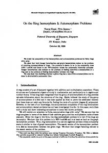
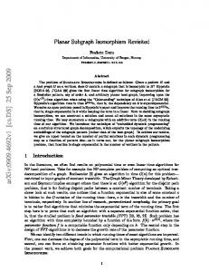
Figure 1: An instance of the subtree isomorphism problem. The tree G has a subtree which is isomorphic to H. every p ≥ 2, if we also add the restriction that G is p-connected, or that H has bounded degree [33]. A faster algorithm for the former case was given in [11]. The subgraph isomorphism problem is also polynomial on planar graphs, or more generally, on the family of graphs with no K3,a minor for every fixed a [14]. In this paper we study the subtree isomorphism problem, i.e., the subgraph isomorphism problem when G and H are trees. Figure 1 gives an instance of this problem. The subgraph isomorphism and the subtree isomorphism problems have applications in pattern recognition, computational biology, and chemistry [3, 37, 41]. Throughout this work, n and k denote the number of vertices in G and H, respectively. When k = n we get the tree isomorphism problem, which has a linear time algorithm due to Hopcroft and Tarjan [23]. Polynomial algorithms for subtree isomorphism were first given by Matula [34] and by Edmonds (cf. [35]). Faster algorithms were given by Matula [35] and Chung [7]. The time complexity of Chung’s algorithm is O(k 1.5 n). Furthermore, the subtree isomorphism problem is in RNC, namely, it can be solved by a randomized parallel algorithm in log O(1) n time [18, 25], and the problem on a restricted family of trees is in LOGSPACE and hence in NC [19]. In contrast, the subgraph isomorphism problem is NP-hard when G is a tree and H is a forest (subforest isomorphism [17]). The subtree isomorphism problem on rooted trees is as follows: Given two rooted trees G and H, find a subgraph G0 of G (whose root is the root of G) such that there is an isomorphism between H and G0 that maps √ the root of H to the 0 1.5 root of G . This problem can be solved in O(min(k , kn log log n/ log n) · n) time [28]. A similar problem is the tree pattern matching problem [5, 8, 9, 13, 21, 27, 32]: The input is two rooted trees G, H with an order on the children of every vertex in the trees. The goal is to find a 1-1 mapping f from the vertices of H into the vertices of G such that for every vertex v in H, the i-th child of v is mapped to the i-th child of f (v). The tree pattern matching problem can be

2

solved in n logO(1) k time [8]. Several generalizations of the subtree isomorphism problem have been studied. In the largest common subtree problem, the input is trees G1 , . . . , Gl , and the goal is to find a tree H with the maximum number of vertices, such that each Gi contains a subgraph that is isomorphic to H. The problem for two trees is polynomial (and in RNC), while it is NP-hard for three or more trees [1]. Approximation algorithms for this problem were given in [2, 26]. Another generalization is the maximum subforest problem: Finding a subforest of a given tree with the maximum number of edges which does not contain a subgraph isomorphic to any tree from a given set of trees. The maximum subforest problem was studied in [39]. Our main result is an O((k 1.5 / log k)n)-time algorithm. Our algorithm, like most previous studies of the problem, is based on the close relationship between subtree isomorphism and maximum matching in bipartite graphs. The subtree isomorphism problem is recursively translated into a collection of smaller subtree isomorphism problems, which are solved using maximum matching algorithms. The improved complexity is achieved by a combinatorial lemma that bounds the possible number of distinct subtrees involved, and by using the notion of clique partition and its application by Feder and Motwani to finding maximum matching in bipartite graphs [16]. We show that for the matching problem resulting from the subtree isomorphism problem, we can find a clique partition in a simple way. The ideas we use here also give an improved algorithm for the maximum subforest problem [39]. We also give a randomized (Las Vegas) algorithm for the decision problem whose expected running time is O(k ω−1 n), where ω is the exponent of matrix multiplication. Using the best known bound for ω [10], the above bound is O(k 1.376 n). This algorithm follows directly from a randomized algorithm for finding the cardinality of a maximum matching given by Cheriyan [6]. The results in this chapter were published in [38] and [40]. The rest of the paper is organized as follows: Section 2 describes an O(k 1.5 n) algorithm for subtree isomorphism. In Section 3 we prove some simple lemmas on matching that are needed in later sections. In Section 4 we prove the combinatorial lemma and use it together with the clique partition in order to improve the running time of the algorithm from Section 2. Finally, Section 5 describes the randomized algorithm. We finish this section with some definitions. For more definitions and basic graph terminology see, e.g., [4]. A rooted tree is a triplet G = (V, E, r), where (V, E) is an unrooted tree, and r is some vertex in V which is called the root. We will sometimes write Gr to denote that r is the root of the rooted tree G. Also, for an unrooted tree G, we denote by Gr the rooted tree formed by choosing the vertex r to be its root. We denote by Grv the rooted subtree of Gr whose vertices are all descendants of v, and its root is v. We say that two rooted trees Gr and H s are isomorphic if there is an iso3

morphism between G and H which maps r to s. Likewise, we write H s ⊆R Gr if there is a rooted subtree J r of Gr which is isomorphic to H s (note that the subtree J r must have the same root as Gr ). We define the open neighborhood of a vertex v in a graph G by N (v) = {u : uv ∈ E}, and the closed neighborhood by N [v] = N (v) ∪ {v}. We use dG (v) to denote the degree of a vertex v in a graph G (or d(v) if G is clear from the context).

2

An O(k 1.5n) algorithm

In this section we describe an O(k 1.5 n) algorithm for the subtree isomorphism problem that will be the basis for the improved algorithms in sections 4 and 5. It is based on Chung’s algorithm [7] and has the same asymptotic time complexity, but is simpler as the tree G is traversed only once, compared to twice in Chung’s algorithm. We briefly describe the algorithm for completeness. We note that the improvements of sections 4 and 5 can also be applied to Chung’s original algorithm. For simplicity, we describe an algorithm for the decision problem. It can be extended easily to an algorithm for the search problem. Let G = (V, E) and H = (VH , EH ) be the input trees (w.l.o.g. |VH | > 1). Select a vertex r of G to be the root. We wish to know for each v ∈ V and u ∈ VH whether H u ⊆R Grv . In order to compute this efficiently we also need to know for each neighbor w of u if Huw ⊆R Grv (notice that Huw is the graph formed by removing Hwu from H u ). This information is relevant because H u ⊆R Grv iff for every child u0 of u there is a distinct child v 0 of v such that Huu0 ⊆R Grv0 . More generally, we have the following lemma: Lemma 2.1. For every vertex v in Gr , vertex u in H, and a vertex w ∈ N [u], we have that Huw ⊆R Grv iff for every child u0 of u in Huw there is a distinct child v 0 of v such that Huu0 ⊆R Grv0 . We store this information in sets S(v, u) defined as follows: For every v ∈ V , and for every u ∈ VH , S(v, u) = {w ∈ N [u] : Huw ⊆R Grv }.

See Figure 2 for an example for this definition. Notice that (1) u ∈ S(v, u) if and only if H u = Huu ⊆R Grv , (2) u ∈ S(v, u) implies S(v, u) = N [u], and (3) d(v) < d(u) − 1 implies S(v, u) = φ. The algorithm computes the sets S(v, u) for all v and u. We show how to compute S(v, u) inductively by going over the vertices v of Gr from the leaves to the root and computing S(v, u) for all u ∈ VH (the algorithm is also described using pseudo-code in Figure 3). The base of the induction is when v is a leaf of Gr . Then S(v, u) can be computed for all u as follows: If u is a leaf of H, then S(v, u) consists of one vertex which is the single neighbor of u in H. Otherwise, if u is an internal vertex, S(v, u) is empty. 4

Sfrag replacements

r G

r

H u

v v1

v2

B(v, u)

v3

u1

u2

v1

v2

v3

u1

u2

u3

u3

Figure 2: An instance of subtree isomorphism. Here, we have H u , Huu2 6⊆R Grv and Huu1 , Huu3 ⊆R Grv , so S(v, u) = {u1 , u3 }. The graph B(v, u) is the bipartite graph which we construct in order to compute S(v, u). There is an edge ui vj in this graph iff u ∈ S(vj , ui ). H u 6⊆R Grv as B(v, u) does not contain a matching of size 3. Huu1 ⊆R Grv as Bu1 (v, u) = B(v, u) − u1 contains a matching of size 2. For the inductive step, consider an internal vertex v (from (3) we can assume that d(v) ≥ d(u)−1). We first need to compute S(v 0 , u) for all the children v 0 of v, for all u ∈ VH . Then, in order to decide for w ∈ N [u] if w ∈ S(v, u), we construct a bipartite graph Bw (v, u) with the two parts Xwv,u and Y v,u , where Xwv,u is the set of children of u in Huw , Y v,u is the set of children of v, and u0 v 0 is an edge of Bw (v, u) iff Huu0 ⊆R Grv0 (i.e., iff u ∈ S(v 0 , u0 )). By Lemma 2.1, w is in S(v, u) iff Bw (v, u) has a matching of size |Xwv,u |. Therefore, in order to compute S(v, u) we need to find maximum matchings in d(u) + 1 bipartite graphs. However, all these graphs are similar one to another: Each graph Bw (v, u) (for w 6= u) is obtained by deleting the vertex w from the graph Bu (v, u). In Section 3 (Corollary 3.2) we shall show that it suffices to find a maximum matching only in Bu (v, u), and then we can efficiently compute the size of the maximum matching in Bw (v, u) for all w 6= u. In the following, we will use B(v, u) instead of Bu (v, u). See Figure 2 for an example of the relation between S(v, u) and the graph B(v, u). Algorithm Subtree-Isomorphism is described by the pseudo-code shown in Figure 3. Theorem 2.2. Algorithm Subtree-Isomorphism solves the subtree isomorphism problem in O(k 1.5 n) time and O(kn) space. Proof. The correctness of the algorithm follows from Lemma 2.1. Let us consider the space complexity. Let V = {x1 , . . . , xn }, and VH = {y1 , . . . , yk }. As each set S(v, u) is a subset of N [u], we can maintain S(v, u) using a binary vector A(v, u) of size |N [u]|. Also, we maintain a k × k matrix I, where I(u, w) is the index of w ∈ N [u] in the vector A(v, u). In other words, w ∈ S(v, P u) iff bit number I(u, w) in A(v, u) is set. Thus the space complexity is O(k 2 + kj=1 d(yj )n) = O(kn) and each access to S(v, u) takes constant time. 5

1 2 3 4 5 6 7 8 9

Select a vertex r of G to be the root of G. For all u ∈ H, v ∈ G do S(v, u) ← φ. For all leaves v of Gr do For all leaves u of H do S(v, u) ← N (u). For all internal vertices v of Gr in a postorder do Let v1 , . . . , vt be the children of v. For all vertices u = u0 of H with degree at most t + 1 do Let u1 , . . . , us be the neighbors of u. Construct a bipartite graph B(v, u) = (X, Y, Evu ), where X = {u1 , . . . , us }, Y = {v1 , . . . , vt }, and Evu = {ui vj : u ∈ S(vj , ui )}. Denote X0 = X and Xi = X − {ui }. 10 For all 0 ≤ i ≤ s do compute the size mi of a maximum matching between Xi and Y . 11 S(v, u) ← {ui : mi = |Xi |, 0 ≤ i ≤ s}. 12 If u ∈ S(v, u) then answer YES and stop 13 end for 14 end for 15 Answer NO. Figure 3: Algorithm Subtree-Isomorphism(G, H).

6

As for the algorithm’s time complexity, the crux is step 10. It computes the size of several maximum matchings in some graphs. Since these graphs are very related to each other, we are able to show in Section 3 that computing the sizes of their maximum matchings can be done in the same time bound taken by computing a single maximum matching. We therefore perform step 10 of the algorithm using Corollary 3.2, and therefore the dominant part of the algorithm’s time complexity is finding maximum matchings in the graphs B(xi , yj ) for all i, j in step 10. Finding a maximum matching in B(xi , yj ) takes O(d(yj )1.5 d(xi )) time using the algorithm of Hopcroft and Karp [22] (or the equivalent algorithm ofP Dinic [12]) and therefore the time needed to handle a vertex xi is at most O( kj=1 d(yj )1.5 d(xi )) = O((2k)1.5 d(xi )). Thus, the total time complexity is O(k 1.5 n). We note that the above algorithm can be changed to solve the subtree homeomorphism problem without changing the asymptotic complexity. The same modification applies to the algorithms in the sections below.

3

Matching

In this section, we give several lemmas about matchings which are needed for obtaining the more efficient algorithms for the subtree isomorphism problem. For the following lemmas, let B = (X, Y, E) be a bipartite graph, where X = {x1 , . . . , xs }, Y = {y1 , . . . , yt } and s ≤ t + 1. Denote X0 = X and Xi = X − {xi } for 1 ≤ i ≤ s. For 0 ≤ i ≤ s, let mi denote the size of a maximum matching between Xi and Y . Clearly for every i ≥ 1, either mi = m0 or mi = m0 − 1. An important notion in matching theory is critical vertices (see, e.g., [31]): A vertex x in a graph G is critical if the size of a maximum matching in G − x is strictly less than the size of a maximum matching in G (i.e., xi is critical iff mi = m0 − 1). Let M be a maximum matching of B. We define a directed graph BM by BM = (X ∪ Y, EM ) where EM = {(x, y) : xy ∈ E − M, x ∈ X, y ∈ Y } ∪ {(y, x) : xy ∈ M, x ∈ X, y ∈ Y }. We denote by XM all the vertices from X which are unmatched in M . Lemma 3.1. For every maximum matching M of B and every vertex xi ∈ X, xi is critical (i.e. mi = m0 − 1) if and only if xi is matched in M , and there is no directed path in BM from a vertex in XM to xi . Proof. (→) The proof is by contradiction. If xi is unmatched in M , then M is a matching between Xi and Y and therefore mi = m0 , a contradiction. Also, if there is a path P in BM from a vertex in XM to xi , then M 4 P (= M ∪ P − M ∩ P ) is a maximum matching in which xi is unmatched, and again we have a contradiction as mi = m0 . 7

(←) Conversely, assume by contradiction that mi = m0 . Let y be the vertex matched to xi in M . As |M − {xi y}| = m0 − 1 < mi , M − {xi y} is not a maximum matching between Xi and Y , and by Berge’s theorem (see [31]) there is an augmenting path P whose one end is a vertex xj ∈ XM , and the other end is y (because if the other end is a vertex in Y that is unmatched in M then P is an augmenting path for M ). But this implies a directed path in BM from xj to xi , a contradiction. Corollary 3.2. Given a maximum matching M of B, we can compute the value of mi for 0 ≤ i ≤ s in O(st) time. Proof. Building the graph BM and finding all the vertices reachable from XM can be done in O(st) time using a depth-first search [42]. We then apply Lemma 3.1. For each vertex xi , if xi is matched in M and is not reachable from XM we set mi = |M | − 1 and otherwise mi = |M |. Lemma 3.3. The problem of finding a maximum matching in B can be reduced in O(st) time to the problem of finding a maximum matching in a subgraph of B with at most s2 vertices and edges and with maximum degree at most s. Proof. Let X 0 be the set of all vertices of X with degree less than s. Let B 0 be the subgraph induced from B by the vertices of X 0 and their neighbors. Building X 0 and B 0 takes O(|X| + |Y | + |E|) = O(st) time. We claim that given a maximum matching M 0 of B 0 we can build a maximum matching M of B: First, add all the edges of M 0 to M . For each vertex x ∈ X − X 0 find an unmatched neighbor y ∈ Y and add xy to M (such a vertex y must exist since each such x has at least s neighbors and at most s − 1 of them are matched). Finding an unmatched neighbor of x takes O(s) time, and therefore building M takes O(s2 ) time.

4

1.5

k An O( log n) algorithm k

We now improve the algorithm from Section 2 by a log k factor. We use the previous algorithm but we solve the maximum matching problems more efficiently using the idea of clique partition of a bipartite graph and its usage in finding maximum matching [16]. The algorithm of Feder and Motwani, originally stated for bipartite graphs with equal size parts, can be extended to general bipartite graphs. This allows one to give an algorithm for subtree isomorphism whose time complexity is O((k 1.5 / log k)n). Instead of describing the modifications to the algorithm of Feder and Motwani, we will give here a simpler way for obtaining an O((k 1.5 / log k)n)-time algorithm for subtree isomorphism. In contrast with [16] where the denseness of the graph is exploited, we achieve the reduction in time complexity by utilizing the special structure of the matching problems that must be solved in the subtree isomorphism algorithm. 8

The modified algorithm, called Improved-Subtree-Isomorphism, is the same as the algorithm Subtree-Isomorphism with the exception that, in step 10, we solve the maximum matching problems differently. Let v be some vertex in Gr whose children are v1 , . . . , vt , and let u be a vertex in H whose neighbors are u1 , . . . , us . We now consider finding a maximum matching in B = B(v, u). Recall that B = (X, Y, E) with X = {u1 , . . . , us } and Y = {v1 , . . . , vt }. We assume that s ≤ t + 1 (because otherwise S(v, u) = φ). We first apply Lemma 3.3 and build a subgraph B 0 = (X 0 , Y 0 , E 0 ) of B having maximum degree at most s. Then, like in [16], we partition the edges of B 0 into complete bipartite graphs C1 , . . . , Cp . We do the partition in the following way: First, we sort the vertices of X 0 in lexicographic order where the key of a vertex u is N (u). Afterward, we split X 0 into sets of equal keys X 1 , . . . , X p (i.e., all the vertices in a set X i have the same neighbors in Y 0 ). Now, for 1 ≤ i ≤ p we set Ci to be the subgraph induced by the vertices of X i and all their neighbors in Y 0 . We now follow the method of [16] and build a network B ∗ whose vertices are V ∗ = X 0 ∪ Y 0 ∪ {c1 , . . . , cp , a, b}. The edges are E ∗ = E1 ∪ E2 , where E1 = {aui : ui ∈ X 0 } ∪ {vi b : vi ∈ Y 0 } E2 = {ui cj : j ≤ p, ui ∈ Cj } ∪ {cj vi : j ≤ p, vi ∈ Cj }

All edges have capacity 1. The source is a and the sink is b. We find a maximum (integral) flow f in B ∗ using Dinic’s algorithm [12] (see also [15]), and construct from this flow a maximum matching in B 0 . (Since the capacity of all edges is 1, the flow f can be decomposed into edge-disjoint paths from a to b where the flow along each path is 1. Since each such path is of the form [a, ui , ck , vj , b], we can define a matching in B 0 by taking the edge ui vj for each such path. The maximality of this matching follows from the maximality of the flow.) We will now analyze the time complexity of the algorithm described above. We denote by D(u) the number of distinct trees in the forest Huu1 , . . . , Huus . Lemma 4.1. Algorithm Improved-Subtree-Isomorphism finds a maximum matching in B(v, u) in O(st + ts0.5 D(u)) time. Proof. Note that if for some i, j the rooted trees Huui and Huuj are isomorphic, then in B = B(v, u) the vertices ui , uj have exactly the same neighbors, and this remains true in B 0 (assuming that ui and uj were not deleted in B 0 ). Therefore p ≤ D(u). The time for constructing B, B 0 , and B ∗ is O(st) (we sort the vertices of X 0 using radix-sort). We now bound the time for finding a maximum flow in B ∗ : The size of E1 is |X 0 | + |Y 0 |, where |X 0 | ≤ s and |Y 0 | ≤ sp (since each vertex in Y 0 has at least one edge arriving from some vertex cj , and no more than s edges depart from each vertex cj to the vertices in Y 0 ). The size of E2 is at most 2sp as the number of edges in E2 incident on some vertex cj is at most |X 0 | + dB 0 (ui ) ≤ 2s where ui ∈ Cj . Hence, the number of edges in B ∗ is O(sp). 9

The number of vertices in B ∗ is atp most s + t + p + 2 = O(t) (as s ≤ t + 1). Now, Dinic’s algorithm performs O( |V ∗ |) stages (see [16]), and each stage takes O(|E ∗ |) time. Hence, the total time is O(t0.5 sp) = O(ts0.5 p) = O(ts0.5 D(u)). We denote again V = {x1 , , . . . , xn } and VH = {y1 , , . . . , yk }. By Lemma 4.1, the time complexity of algorithm Improved-Subtree-Isomorphism is O(

n X k X

0.5

(d(yj )d(xi ) + d(xi )d(yj ) D(yj ))) = O(kn + n

i=1 j=1

k X

d(yj )0.5 D(yj )).

j=1

P We will bound the summation kj=1 d(yj )0.5 D(yj ) by O(k 1.5 / log k). We first need a simple combinatorial lemma. Let g(n) denote the number of distinct (i.e., non-isomorphic) rooted trees with n vertices. We shall use the following result: Lemma 4.2. (see, e.g., [36, p. 1197]) g(n) = 2Θ(n) . Let f (n) denote the maximum number of distinct rooted trees in a forest with n vertices. Lemma 4.3. f (n) = Θ(n/ log n). Proof. To show the lower bound, we use the fact that g(n) ≥ 2n for large n. Hence, the number of distinct rooted trees with l = blog logn n c vertices is g(l) ≥ n

n n 2log log n −1 = 2 log . Therefore we can build a forest by taking b 2 log c distinct trees n n n with l vertices each, and the total number of vertices in this forest is b 2 log cl < n. n n Thus f (n) = Ω( log n ). We will now show the upper bound. If we have a forest of rooted trees and ri is the number of trees Pn with i vertices, then the number of distinct trees in this forest is at most i=1 min(ri , g(i)). Hence, ) ( n n X X iri ≤ n . f (n) ≤ max min(ri , g(i)) : r1 , . . . , rn ∈ , i=1

i=1

By Lemma 4.2, f (n) ≤ max

( n X i=1

i

min(ri , c ) : r1 , . . . , rn ∈

,

n X i=1

iri ≤ n

)

P for some integer constant c. Let x be the minimum which xi=1 ici ≥ n. Pn integer for i Let Pn r1 , . . . , rn be the integers that maximizei i=1 min(ri , c ) under the jconstraint c for all i, because if rj > c for some i=1 iri ≤ n. We can assume that ri ≤P j j, we can set rj = c and the value of ni=1 min(ri , ci ) does not change. Now, suppose that rj > 0 for some j > x. This implies that there is a k ≤ x for which 10

P P P rk < ck (because otherwise ni=1 iri ≥ xi=1 iri + jrj = xi=1 ici + jrj > n, a contradiction). If we decrease rj by one, and increase rkP by one, then the value Pn i of i=1 min(ri , c ) does not change, and the constraint ni=1 iri ≤ n still holds (as k < j). We can repeat this process until rj = 0 for all j > x and therefore f (n) ≤

n X i=1

i

min(ri , c ) ≤

x X

ci = O(cx ).

i=1

The lemma follows from the fact that x = logc n − logc logc n + O(1). We now continue with the analysis of algorithm Improved-Subtree-Isomorphism. Let  be some constant 0 <  < 1/3. We call a vertex of H heavy if its degree is at least 2k 1− , and otherwise it is called light. Clearly, the number of heavy vertices is at most k  . If u is a heavy vertex and v is a neighbor of u such that Hvu does not contain a heavy vertex, then we call every vertex in Hvu a private vertex of u. We denote by lj the number of the private vertices of a heavy vertex yj . Lemma 4.4. For every heavy vertex yj , d(yj ) ≤ k  + lj and D(yj ) ≤ k  + f (lj ). Proof. Let u1 , . . . , up denote the neighbors of yj which are private vertices of yj and let v1 , . . . , vq denote the rest of the neighbors of yj . Clearly, p is at most the total number of private vertices of yj which is lj . Furthermore, for each y vertex vi we can chose a heavy vertex wi in Hvij . As the vertices we chose are distinct, we have that q is less than the number of heavy vertices. Hence, d(yj ) = q + p ≤ k  + lj . y y The trees Hu1j , . . . , Hupj constitute all the private vertices of yj , and therefore they have a total of lj vertices and there are at most f (lj ) distinct trees among them. Hence, D(yj ) ≤ q + f (lj ) ≤ k  + f (lj ). P Lemma 4.5. kj=1 d(yj )0.5 D(yj ) = O(k 1.5 / log k).

P Proof. We split kj=1 d(yj )0.5 D(yj ) into two sums. Summing over the light vertices of H we have X X X d(yj )0.5 D(yj ) ≤ d(yj )1.5 ≤ (2k 1− )0.5 d(yj ) j:yj is light

j:yj is light

j:yj is light

≤ (2k 1− )0.5 2k = 21.5 k 1.5−/2 ,

P where the last inequality follows from the fact that kj=1 d(yj ) = 2k − 2. Summing over the heavy vertices and using Lemma 4.4 we have X X d(yj )0.5 D(yj ) ≤ (k /2 + lj0.5 )(k  + f (lj )). j:yj is heavy

j:yj is heavy

11

Since f (lj ) ≤ lj ≤ k and since the number of heavy vertices is at most k  , we have X (k 3/2 + k 0.5+ + k 1+/2 + lj0.5 f (lj )) ≤ j:yj is heavy

≤ 3k 1+3/2 +

X

lj0.5 f (lj )

j:yj is heavy

P and by Lemma 4.3, the fact that j:yj is heavy lj ≤ k (as each vertex can be a private vertex of at most one heavy vertex), and the fact that the function h(x) = x1.5 / log x is convex, ≤ 3k

1+3/2

+ j:yj

lj1.5 k 1.5 c . ≤ 3k 1+3/2 + c log lj log k is heavy

X

We therefore proved the following theorem: Theorem 4.6. Algorithm Improved-Subtree-Isomorphism solves the subtree isomorphism problem in O((k 1.5 / log k)n) time.

5

An O(k 1.376 n) algorithm

In this section we give a randomized algorithm for the decision problem of subtree isomorphism. The algorithm is more efficient asymptotically than the deterministic algorithm of the previous section. Again, the algorithm Randomized-Subtree-Isomorphism is based on the algorithm Subtree-Isomorphism but solving the maximum matching problems is done differently. Consider some vertex v in Gr whose children are v1 , , . . . , vt , and some vertex u in H whose neighbors are u1 , . . . , us . We use the algorithm of Cheriyan [6] to find the size of a maximum matching in B(v, u) and to find all the critical vertices in B(v, u). Cheriyan’s algorithm for finding critical vertices (in a general graph) is as follows: Given an input graph G = (V, E), where V = {1, 2, . . . , n}, choose a large prime number q and build an n × n matrix C in the following way: For each edge ij ∈ E, choose a random number wij uniformly from {1, 2, . . . , q − 1}, and set cij = wij and cji = −wij . Set all the other elements of C to zero. Finally, find a basis a1 , . . . , ar for the null space of C over the field Zq . Then, with high probability, the size of a maximum matching in G is equal to (n − r)/2 and for all i ∈ V , vertex i is critical iff all the i-th coordinates of a1 , . . . , ar are zeros. As the graph B(v, u) is bipartite, when applying Cheriyan’s algorithm on B(v, u), the matrix C is of the form   0 C0 C= , C 00 0 12

where C 0 is a t × s block and C 00 is an s × t block. Therefore, we can find a basis for the null space of C by finding bases for the null spaces of C 0 and C 00 . This can be done in O(sω−1 t) time [24], where ω denotes the exponent of matrix multiplication. P Thus, P the running time of algorithm Randomized-SubtreeIsomorphism is O( ni=1 kj=1 d(yj )ω−1 d(xi )) = O(k ω−1 n). Theorem 5.1. Algorithm Randomized-Subtree-Isomorphism solves the decision problem in O(k ω−1 n) expected time. Since ω < 2.376 [10], we have Corollary 5.2. Algorithm Randomized-Subtree-Isomorphism solves the decision problem in O(k 1.376 n) expected time.

6

Acknowledgment

We are grateful to the anonymous referee for a careful reading of the manuscript and many helpful comments.

References [1] T. Akutsu. An RNC algorithm for finding a largest common subtree of two trees. IEEE Trans. Information Systems, E75-D:95–101, 1992. [2] T. Akutsu and M. M. Halld´orsson. On the approximation of largest common subtrees and largest common point sets. In Proc. 5th Int. Symposium on Algorithms and Computation, LNCS 834, pages 405–413. Springer-Verlag, 1994. [3] S. Anderson. Graphical representation of molecules and substructure-search queries in MACCS. J. of Molecular Graphics, 2:8–90, 1984. [4] M. Behzad, G. Chartrand, and L. Lesniak-Foster. Wadsworth International Group, 1979.

Graphs & Digraphs.

[5] C. Chauve. Pattern matching in static trees. Research Report RR 1254-01, LaBRI Univ. Bordeaux, 2001. ˜ (|V |)) algorithms for problems in matching [6] J. Cheriyan. Randomized O(M theory. SIAM J. Computing, 26:1635–1655, 1997. [7] M. J. Chung. O(n2.5 ) time algorithms for the subgraph homeomorphism problem on trees. J. of Algorithms, 8:106–112, 1987.

13

[8] R. Cole and R. Hanharan. Tree pattern matching and subset matching in randomized O(n log3 m) time. In Proc. 29th Symposium on the Theory of Computing (STOC 97), pages 66–75, 1997. [9] R. Cole, R. Hanharan, and P. Indyk. Tree pattern matching and subset matching in deterministic O(n log3 n)-time. In Proc. 10th Symposium on Discrete Algorithms (SODA 99), pages 245–254, 1999. [10] D. Coppersmith and S. Winograd. Matrix multiplication via arithmetic progressions. J. Symbolic Comp., 9:23–52, 1990. [11] A. Dessmark, A. Lingas, and A. Proskurowski. Faster algorithms for subgraph isomorphism of k-connected partial k-trees. Algorithmica, 27(3):337– 347, 2000. [12] E. A. Dinic. An algorithm for solution of a problem of maximum flow in a network with power estimation. Soviet Math. Doklady, 11:1277–1280, 1970. [13] M. Dubiner, Z. Galil, and E. Magen. Faster tree pattern matching. In Proc. 31st Symposium on Foundation of Computer Science (FOCS 91), pages 145– 149, 1990. [14] D. Eppstein. Subgraph isomorphism in planar graphs and related problems. In Proc. 6th Symposium on Discrete Algorithms (SODA 95), pages 632–640. ACM press, 1995. [15] S. Even. Graph Algorithms. Computer Science Press, Rockville, Maryland, 1979. [16] T. Feder and R. Motwani. Clique partitions, graph compression and speeding-up algorithms. In Proc. 23rd Symposium on the Theory of Computing (STOC 91), pages 123–133. ACM press, 1991. [17] M. R. Garey and D. S. Johnson. Computers and Intractability: A Guide to the Theory of NP-Completeness. W. H. Freeman and Co., San Francisco, 1979. [18] P. B. Gibbons, R. M. Karp, G. L. Miller, and D. Soroker. Subtree isomorphism is in random NC. Discrete Applied Math, 29:35–62, 1990. [19] R. Greenlaw. Subtree isomorphism is in DLOG for nested trees. Int. J. of Foundations of Computer Science, 7:161–167, 1996. [20] A. Gupta and N. Nishimura. Characterizing the complexity of subgraph isomorphism for graphs of bounded path-width. In Proc. 17th Int. Symp. Theoretical Aspects of Computer Science (STACS 96), LNCS 1046, pages 453–464. Springer-Verlag, 1996. 14

[21] C. M. Hoffmann and M. J. O’Donnell. Pattern matching in trees. J. Assoc. Comput. Mach., 29(1):68–95, 1982. [22] J. E. Hopcroft and R. M. Karp. A n5/2 algorithm for maximum matching in bipartite graphs. SIAM J. Computing, 2:225–231, 1973. [23] J. E. Hopcroft and R. E. Tarjan. Isomorphism of planar graphs. In Raymond E. Miller and James W. Thatcher, editors, Complexity of Computer Computations, pages 131–152. Plenum Press, 1972. [24] O. H. Ibarra, S. Moran, and R. Hui. A generalization of the fast LUP matrix decomposition algorithm and applications. J. of Algorithms, 3:45–56, 1982. [25] M. Karpinski and A. Lingas. Subtree isomorphism is NC reducible to bipartite perfect matching. Information Processing Letters, 30(1):27–32, 1989. [26] S. Khanna, R. Motwani, and F. F. Yao. Approximation algorithms for the largest common subtree problem. Technical Report STAN-CS-95-1545, Stanford University, Dept. Computer Science, 1995. [27] S. R. Kosaraju. Efficient tree pattern matching. In Proc. 30th Symposium on Foundation of Computer Science (FOCS 89), pages 178–183, 1989. [28] A. Lingas. An application of maximum bipartite C-matching to subtree isomorphism. In Proc. 8th Colloquium on Trees in Algebra and Programming (CAAP 83), LNCS 159, pages 284–299. Springer-Verlag, 1983. [29] A. Lingas. Subgraph isomorphism for biconnected outerplanar graphs in cubic time. Theoretical Computer Science, 63:295–302, 1989. [30] A. Lingas and M. M. Syslo. A polynomial-time algorithm for subgraph isomorphism of two-connected series-parallel graphs. In Proc. 15th Int. Colloq. Automata, Languages and Programming, LNCS 317, pages 394–409. Springer-Verlag, 1988. [31] L. Lovasz and M. D. Plummer. Matching Theory. North-Holland, Amsterdam, 1986. [32] F. Luccio and L. Pagli. An efficient algorithm for some tree matching problems. Information Processing Letters, 39:51–57, 1991. [33] J. Matouˇsek and R. Thomas. On the complexity of finding iso- and other morphisms for partial k-trees. Discrete Math, 108:343–364, 1992. [34] D. W. Matula. An algorithm for subtree identification. SIAM Rev., 10:273– 274, 1968.

15

[35] D. W. Matula. Subtree isomorphism in O(n5/2 ). Ann. Discrete Math., 2:91– 106, 1978. [36] A. M. Odlyzko. Asymptotic enumeration methods. In R. L. Graham, M. Grotschel, and L. Lovasz, editors, Handbook of Combinatorics, volume 2, pages 1063–1229. Elsevier and the MIT press, 1995. [37] M. Pelillo, K. Siddiqi, and S. W. Zucker. Matching hierarchical structures using association graphs. In H. Burkhardt and B. Neumann, editors, Computer Vision—ECCV 98, LNCS 1407, pages 3–16. Springer-Verlag, 1998. [38] R. Shamir and D. Tsur. Faster subtree isomorphism. In Proc. 5th Israel Symposium on Theory of Computing and Systems, (ISTCS 97), pages 126– 131, 1997. [39] R. Shamir and D. Tsur. The maximum subforest problem: Approximation and exact algorithms. In Proc. 9th Symposium on Discrete Algorithms (SODA 98), pages 394–399. ACM press, 1998. [40] R. Shamir and D. Tsur. Faster subtree isomorphism. J. of Algorithms, 33:267–280, 1999. [41] R. E. Stobaugh. Chemical substructure searching. J. of Chemical Information and Computer Sciences, 25:271–275, 1985. [42] R. E. Tarjan. Depth-first search and linear graph algorithms. SIAM J. Computing, 1:146–160, 1972.

16