FAULT DETECTION OF AN INDUCTION MOTOR BY SET-MEMBERSHIP FILTERING AND KALMAN FILTERING C. Durieu*, L. Loron+, E. Sedda*, I. Zein+ *
LESiR UPRESA, 61 Avenue du Président Wilson, F-94235 Cachan Cedex tél : 33 1 47 40 27 10, fax : 33 1 47 40 21 99
[email protected],
[email protected] + Laboratoire d’Electromécanique, U.T.C. B.P. 20529, F- 60205 Compiègne Cedex tél : 33 3 44 23 45 14, fax : 33 3 44 20 48 13
[email protected],
[email protected]
Keywords: ellipsoidal bounding, fault detection, induction motor, Kalman filtering, set-membership estimation.
Abstract Two approaches are presented in this paper to estimate the state of an induction motor and detect faults: a geometric approach, assuming only that the perturbations belong to known bounded sets with no hypothesis on their distributions inside these sets, and a stochastic approach by Kalman filtering. Recursive and explicit algorithms are presented and illustrated by real data of an induction motor that has been designed to have some more and less important faults.
1 Introduction Estimation techniques are more and more used in fault detection and diagnosis of induction motors [West, Naït]. Most state estimation problems are solved via a stochastic approach. Measurement noise, disturbances and model errors are assumed to be a realization of a random process. These estimation techniques require the knowledge of stochastic characteristics of the different disturbances and a Kalman filter is often used to solve such a problem [Atki, Loro, Deva]. However, in some situations, it can be more natural to consider a geometric approach, assuming only that the perturbations belong to known bounded sets with no hypothesis on their distributions inside these sets. This bounded-error approach describes the set of all the states that are consistent with the model, the data and the error bounds. All elements of this feasible set are then candidate solutions for the estimation problem. The set thus obtained may become extremely complicated. In order to be computed in real time, this feasible set is recursively characterized by the smallest ellipsoid that encloses it [Schw]. Usually, the size of an ellipsoid, characterizing the state estimation uncertainty, is measured by its volume, which is proportional to the square of the product of the semi-axe lengths and corresponds to the determinant criterion. However, this criterion presents some
disadvantages, this is why an alternative criterion, namely the trace criterion which corresponds to the sum of the squares of the semi-axe lengths of the ellipsoid, is also considered [Duri]. In this paper, the fault detection is based on the electrical model of the induction motor. Therefore, the Kalman filter and the set-membership will only detect faults that have a significant effect on the electrical behavior of the motor. Both approaches take into account model approximations and measurement errors to estimate the motor state. To obtain a fault detection with a high sensitivity, these uncertainties must be minimized. Moreover, the working conditions have a large influence on the fault detection sensitivity. For instance, a broken bar cannot be detected if the motor torque is null. Nevertheless, the proposed approaches offer practical advantages: no supplementary instrumentation is required and the state estimation can also be used for the torque control of the motor. To illustrate the behavior of these schemes, realistic electrical faults of the motor, instead of the usual elementary faults (additive or multiplicative faults), are considered in this paper. One of the weakest parts of the induction motor is the stator insulation. Modern static converters produce high electrical strains which may cause insulation failure like turnto-turn short-circuit. The Laboratoire d'Automatique et d'Informatique Industrielle de Poitiers (LAII) has specifically designed an induction motor to simulate electrical failure: the stator winding can be more or less unbalanced by shortening partially one phase. The paper is organized as follows. Models of the motor are specified in Section 2. Algorithms are presented in Section 3 and illustrated in Section 4 to detect faults of the induction motor.
2 Models State estimation is based on a discrete-time varying linear model of the induction motor in the two-phase rotor reference frame. The model assumes sinusoidal magnetomotive forces,
non-saturation of the magnetic circuit and a negligible skin effect. If the mechanical speed ω is assumed to be quasistationary with respect to the dynamics of the electric variables, the model becomes linear but not stationary with four order differential equations. Yamamura has shown that the repartition of the leakage inductance between the stator and the rotor can be arbitrary -chosen, provided that the leakage factor is kept [Yama]. The model of the induction motor is simplified if one chooses a null rotor leakage inductance. Then, the continuous time model, expressed in the mechanical reference frame, is x&( t ) = Ac ( ω )x ( t ) + Bc u( t ) y ( t ) = Cx( t ) (1) with −
Ac =
R s + Rr
pω
L fs − pω
−
Rs + R r L fs
Rr
0
0
Rr
Rr
pω
L fs L r pω − L fs R − r Lr
L fs Rr
0
L fs L r
,
(2)
0 −
T
Rr Lr
1 0 0 0 ,C= 0 1 0 0 .
(3)
The state vector x is composed of the two-phase components of the stator currents (isα , i sβ ) and the rotor flux (φ sα ,φ rβ ):
[
x = isα isβ φ sα φ rβ
]T .
(5)
with Ac ,k = Ac ( ω ( t k )) and tk = kTe (k N ). To take into account discretization errors, model errors, input errors and measurement noise, a process noise vector vk and an observation noise vector w k are added respectively to the state equation and the observation equation of (1) and the discrete-time state model is x k +1 = Ak xk + Bk uk + v k (6) y k = Cx k + wk where x k = x( t k ) and y k = y ( t k ) (k N ). The components of the known input vector u k are the average of the stator voltages between t k and t k + 1 . In this paper, we assume that the different components of the noises are independent. 2.1 Kalman filtering
and 1 1 0 0 0 Bc = L fs 0 1 0 0
1 2 Ak = I + T e Ac,k + ( Te Ac ,k ) 2 1 Bk = T e ( I + T e Ac,k )B c 2
(4)
Kalman filtering assumes that process noise and measurement noise are independent, white and zero-mean random variables with known covariance. The initial state x 0 is assumed to be random with known mean and covariance. Noise wk and noise v k are also assumed to be independent of x 0 . Moreover, if the noise is Gaussian, the Kalman filter is an optimal state estimator with respect to the variance of the estimation error. In practice, the state noise and the observation noise are due to model approximations and measurement noise. Therefore, due to the Central limit theorem, one might expect that the observation noise distribution is roughly Gaussian. More precisely, an analysis with experimental data reveals that the noise is bounded and nearly Gaussian between its bounds that are nearly equal to three times its standard deviation [Loro]. Note that with an exact scalar Gaussian noise, the probability that a noise value belongs to the interval [− 3σ ,3σ ] , where σ is its standard deviation, is equal to 0.997 . Even if the model error is essentially deterministic, to use Kalman filtering, one assumes that it is also stochastic with known standard deviation.
The input vector u( t ) and the output vector y ( t ) are composed respectively of the two-phase stator voltages and the two-phase stator currents. The parameters Rs, L fs , Rr and L r are respectively the stator resistance, the global leakage inductance referred to the stator, the rotor resistance and the rotor inductance. These parameters were previously estimated by an extended Kalman filter from experimental data similar to those of Figure 4.a. The discrete-time model is deduced from the continuous model by a second order serie expansion of the transition matrix. By using a second order serie expansion and the mechanical reference frame, a sampling period of 1 ms can be 2.2 Set membership filtering used. The usual first order serie expansion (Euler approximation) requires a very short sampling period to give With this approach the only information available is that the a stable and accurate model. These approximations by serie state noise v k , the observation noise wk and the initial state expansion are more precise with low frequency signals. Thus, x 0 belong to known compact sets. To reduce complexity, the the mechanical and synchronous reference frames are best v i = 1,L ,4 ) of v k and wk , j suited for the definition of accurate discrete-time models. The different components k ,i ( mechanical reference frame is directly deduced from the rotor ( j = 1,2 ) of wk are assumed to be independent. The noise position measurement. being time-invariant, we can write that Let T e be the sampling period. The second order serie vbounds v′ ≤ 1 = max( v i )v ′k ,i w k , j = max( w j )w′k , j k , i with k ,i and expansion of the transition matrix gives w′ ≤ 1 with k , j . So the equations in (6) can be written as
x k +1 = Ak x k + Bk u k + yk , j
4 i =1
Vi v′k ,i , v ′k ,i ≤ 1 ( i = 1,L ,4 )
(7)
= C j x k + w′k , j , w′k ,j ≤ 1 ( j = 1,2 )
with
V i = max( v i )[δ 1−i , L ,δ 4 −i y k = [max( w 1 ) y k ,1
]T
( i = 1, L ,4 ) ,
(8) (9)
and 1 [1 0 0 0 max( w 1 )
]
C2 =
1 [0 1 0 0 max( w 2 )
]
(14)
and σ k2 ,j = σ 2j + σ k2 / k −1 , j ,
(15)
σ j being the standard deviation of the observation noise and
max(w2 )y k,2 ] ,
C1 =
∆y k , j = y k , j − yˆ k / k −1 , j
.
(10)
Note that the set of all the states x k that satisfy one of the measurement equations of (7), which can be rewritten as y k , j − C j x k ≤ 1 , is a strip. If the components v k ,i or wk , j
σ k / k −1, j the standard deviation of the predicted observation ( j = 1,2 ). The difficulty is then to choose η . According to the previous results, we have takenη = 3 . This value leads theoretically to a rate of false alarm of about 0.3% with exact Gaussian hypothesis. This solution allows real time fault detection. This approach can be completed by a careful analysis of the errors as in [Loro]. 3.2 Set-membership filtering
The aim of the set-membership filter with ellipsoidal approximation is to find recursively the smallest ellipsoid that encloses the feasible set. A recursive algorithm, well adapted to be implemented in real time, can be deviated. More are not independent, then the algorithms to be presented still precisely, bounded error algorithm gives a recursive apply but the approximation obtained will be more ellipsoidal approximation of the uncertainty sets Ω and k/k pessimistic. Ω x n xk and k +1 k +1 / k which enclose respectively all values of Any bounded ellipsoid E of R with a non-empty that are compatible with all available information up to t k, interior can be defined by E(c ,P ) = x R n /( x − c )T P −1 ( x − c ) ≤ 1 , (11) namely the model equations, the error bounds, the initial condition and the measurements y l for . The where c is its center while P is a symmetric positive smallest ellipsoid is computed by minimizing the determinant definite matrix that specifies its size and orientation. The or trace criterion. The initial state space vector x 0 is assumed tr(P) considered measure of the size of E(c ,P ) is for the ˆ E trace criterion and det(P) for the determinant criterion. A to belong to an ellipsoid 0 /0 . The predicted set Ω k +1 / k and the corrected setΩ k +1 / k +1 strip are recursively provided by S(y , d T ) = x R n / y − d T x ≤ 1 (12) 4 Ω k +1 / k = Ak Ω k / k + Bk uk + Vi U is an unbounded ellipsoid that is useful to take into account i= 1 (16) information provided by a scalar measurement. Indeed Ω k +1 / k + 1 = Ω k +1 / k I S(y k +1 ,1 , C1 )I S(y k +1 ,2 ,C 2 ) observation equations of (7) can be rewritten as xk S(yk , j ,C j ) ( j =1,2 ) . with U = [ −1,1 ] . These equations are too complicated to be used in real ˆ time. Let Ek/k be an ellipsoidal approximation of Ω k / k . 3 Algorithms ˆ Ω k +1 / k is approximated by E k +1/k that is the smallest 3.1 Kalman filtering ellipsoid containing 4 For linear system, Kalman filtering gives the linear minimum ˆ +B u + V U Lk +1 = Ak E k /k k k i variance estimate of the state vector. The first step of the , (17) i =1 Kalman algorithm is the state prediction and the second step is the state correction, which takes into account the new which is a weighted sum of ellipsoids. So we have measurements. This approach being classical, the equations ˆ E k+1 /k = arg min tr(Pk+1 / k ) (18) E L k + 1 are not remembered here (Jazw). The fault detection consists in computing a Mahalanobis distance comparing a measurement y k ,j to its predicted value or ˆ - yˆ k / k −1, j = C j ˆx k / k −1 where xˆ k / k −1 is the prediction of xk . E k +1 /k = arg min det (Pk +1 / k ) (19) E L k + 1 More precisely a fault is detected if the following condition is satisfied with E = E(c,P) . Figure 1 illustrates the prediction step for ˆ ∆y k , j > η σ k ,j , (13) the studied application. Ek +1/k +1 is the smallest ellipsoid containing with
{
{
}
}
ˆ I k +1 = E k +1 /k I S(y k +1 ,1 , C 1 )I S(y k +1 , 2 , C 2 ) ,
(20)
that is the intersection of the predicted ellipsoid and the measurement strips. So we have ˆ E (21) k+1 /k +1 = arg min tr (Pk +1 / k ) E I k + 1
or ˆ E k +1 /k +1 = arg min det (Pk +1 / k ) .
(22)
E I k + 1
Figure 2 illustrates the correction step.
ellipsoid center is ordinarily used as a particular estimator of the state. The algorithms are detailed in [Sedd]. The set I k +1 is not empty if the error bounds and the model are correct. If the intersection is empty, a fault or an incoherence due to a model error, underestimated bounds or a faulty sensor is detected. So the bounded technique allows detecting incoherences, but due to the different approximations, we are not guaranteed to detect small faults. If an incoherence is detected, no correction is done and the algorithm is then applied with a new ellipsoid that is large enough to contain the exact state.
-1
4 Experimental results V1 U -1.5
V 2U
Bku k $k k E / $ +B u Ak E k/ k k k
-2
-2.5 -2
-1
-1.5
-0.5
-Fig. 1 - Prediction in the ( isα ,isβ ) plane. 0
S(yk+1,1 ,C1 ) -0.5
I k +1
S(yk+1,2 ,C 2 )
-1
$k +1/k E
$k +1 / k +1 E
-1.5
-2 -2
-1.5
-1
-0.5
Fig. 2 - Correction in the ( i sα , i sβ ) plane.
0
To find the smallest ellipsoids, optimization problems (17, 18, 21 and 22) are solved over parameterized families [Duri] and yield to an explicit solution of the predicted ellipsoid ˆ E k +1/k with the trace criterion, and also an explicit solution with the determinant criterion if the different components of the state noise are recursively introduced. An explicit solution ˆ of Ek +1/k +1 is obt ai ne d if each strip S(y k +1, j , C j ) ( j = 1,2 ) is introduced successively. To obtain a real time algorithm an explicit solution, avoiding optimization problems, is retained at the cost of a suboptimal solution. The
To illustrate the algorithms three examples have been considered: first a motor without fault (Figures 3-a, b and c), then a motor that is a little unbalanced (Figures 4-a, b and c) and then a motor with an important unbalanced fault (Figures 5-a, b and c). The sampling period is equal to 0.7 ms . Voltage inputs, current measurements and speed are plotted on Figures a. The differences ∆y k ,1 and ∆y k ,2 computed by the Kalman filtering can be compared on Figures b with three times their standard deviation, this comparison allowing to detect a fault. Similarly ∆y k ,1 and ∆y k ,2 and their bounds computed by the set-membership filtering with the trace criterion are plotted on Figures c. An incoherence is detected if ∆y k ,1 or ∆y k ,2 is greater than its bound. With the determinant criterion similar results were obtained, so the different curves are not drawn here. As expected, it can be seen in Figure 3.b, that difference ∆y k , j ( j = 1, 2 ) computed by the Kalman filter may occasionally exceed the detection level, even without default. Therefore, to avoid false alarms a sliding window testing several successive data must be considered. On the contrary, Figure 3.c shows that, with the same experiment, the bounded approach offers a suitable margin between the errors and their bounds. With a small stator unbalance, the rate of the large differences increases significantly with the Kalman filter (Figure 4.b) and at times the bounded approach detects incorrect bounds (Figure 4.c). Both algorithms are more sensible during speed transients. With a large unbalance, the Kalman filter continuously detects the fault (Figure 5.b), while the bounded approach detects it only during speed transients (Figure 5.c). These experimental results show the importance of an adequate noise characterization, the influence of the operating conditions and illustrate the feasibility of the algorithms.
stator voltages (V)
stator voltages (V)
400
400
200
200
0
0
-200 0
0.1
0.2
0 .3
0.4
0.5
0.6
0.7
stator currents (A)
0.8
0 .9
1
-200 0
0.1
0.2
0.3
0.4
0.5
0.6
0 .7
0.8
0.9
1
0.8
0.9
1
0.8
0.9
1
stator currents (A)
4
5
2 0
0
-2 -4
0
0.1
0.2
0.3
0.4
0.5
0.6
0.7
0 .8
0.9
1
rotor speed (rad/s)
-5 0 120
0.1
0.2
0.3
0.4
0.5
0.6
0.7
rotor speed (rad/s)
130
1 00
120 110
80
100 90
0
0.1
0.2
0.3
0.4
0.5
0.6
0.7
0.8
0.9
1
60 0
0.1
0.2
0.3
0.4
0.5
time (s)
Fig. 3-a - Motor without fault – Data. |∆y
k,1
| and 3 σ
k,1
0.4
0.4
0.2
0.2
0 0.2
0.3
0.4
0.5
0.6
0.7
| ∆y | and 3σk,2
0.8
0.9
1
0 0
0.6
0.6
0.4
0.4
0.2
0.2 0.1
0.2
0.3
0.4
0.5
0.6
0.7
0.8
0.9
0 0
1
time (s)
0.4
0.4
0.2
0.2 0
0.4
| ∆y
0.5
k,2
0.6
0.7
0.8
0.9
1
1
0.5
0.6
0.7
0.8
0.9
1
0.1
0.2
0.3
0.4
0
0.1
0.2
0.3
0.1
0.2
0.3
| and its bound
0.4
0.5
0.6
0.7
0.8
0.9
1
0.5
0.6
0.7
0.8
0.9
1
| ∆y k,2| and its bound
0.6
0.6
0.4
0.4
0.2
0.2 0
0.9
| ∆yk,1| and its bound 0.6
0.3
0.8
|∆yk,2| and 3 σk,2
Fig. 4-b - Motor with a small fault – Kalman filtering.
0.6
0.2
0.7
0.4
k,1
0.1
0.6
0.3
| ∆y | and its bound
0
0.5
0.2
k,1
time (s)
Fig. 3-b - Motor without fault – Kalman filtering.
0
| and 3 σ
0.1
k,2
0 0
|∆y
k,1
0.6
0.1
0.7
Fig. 4-a - Motor with a small fault – Data.
0.6
0
0.6
time (s)
0 0
0.1
0.2
0.3
0.4
0.5
0.6
0.7
0.8
0.9
time (s)
Fig. 3-c - Motor without fault – Bounded approach.
1
0
0.4
time (s)
Fig. 4-c - Motor with a small fault – Bounded approach.
stator voltages (V)
200
5 Conclusions
100
The results reported here indicate that both the bounded approach and the Kalman filtering are able to detect electrical faults of an induction motor. These algorithms require an adequate noise characterization to be efficient. To take into account natural variations of the electrical parameters (essentially due to the temperature influence) adaptive schemes have to be implemented. This can be obtained with an extended Kalman filter or by a similar extension of the setmembership filtering.
0
-100 -200 0
0.1
0.2
0.3
0.4
0.5
0.6
0.7
0.8
0 .9
1
0.9
1
stator currents (A) 6
4
2 0 -2
0
0.1
0.2
0.3
0.4
0.5
0.6
0.7
0.8
rotor speed (rad/s) 100
Acknowledgements
80 60 40
0
0.1
0.2
0.3
0.4
0.5
0.6
0.7
0.8
0.9
1
time (s)
Fig. 5-a - Motor with important fault – Data. |∆y
k,1
| and 3 σ
The work presented in this paper has been done within the collaboration of three C.N.R.S. Research Groups: "Automatique", "ISIS" and "SDSE". We wish to thank the Laboratoire d'Automatique et d'Informatique Industrielle de Poitiers for the experimental data. This work was partially supported by the Conseil Régional de Picardie.
k,1
0.6
References
0.4
[Atki]
0.2
0 0
0.1
0.2
0.3
0.4
|∆y
0.5
0.6
0.7
| and 3 σk,2
0.8
0.9
1
[Duri]
k,2
0.6
[Deva]
0.4
0.2 0 0
0.1
0.2
0.3
0.4
0.5
0.6
0.7
0.8
0.9
1
[Jazw]
time (s)
Fig. 5-b - Motor with important fault – Kalman filtering.
[Loro]
|∆yk,1| and its bound
[Naït]
0.6
0.4 0.2 0
0
[Schw] 0.1
0.2
0.3
0.4
0.5
0.6
0.7
| ∆y | and its bound
0.8
0.9
1
[Sedd]
k,2
0.6
[West]
0.4 0.2 0 0
[Yama] 0.1
0.2
0.3
0.4
0.5
0.6
0.7
0.8
0.9
1
time (s)
Fig. 5-c - Motor with important fault – Bounded approach.
D.J. Atkinson et al. "Observers for induction motor state and parameter estimation", IEEE trans. on industry applications, vol. 27, n°6, pp. 1119-1127 (1991). C. Durieu, B. Polyak, E. Walter, "Trace versus determinant in ellipsoidal outer-bounding, with application to state estimation", 13th IFAC World Congress, San Francisco, vol I, pp. 43-48 (1996). V. Devanneaux, "Etude et implantation d’un filtre de Kalman en vue de la reconstruction d’état et de l’estimation de paramètres de la machine asynchrone", DEA PARIS VI, LESiR (1997). A. H. Jazwinski, "Stochastic Processes and Filtering Theory", Academic Press (1970). L. Loron, E. Le Carpentier, "Experimental noise characterization for induction motor identification", ELECTRIMACS 96, St Nazaire, Vol. 2, pp; 787-79 (1996). M.S. Naït Saïd et al. "Sensorless induction motors failure monitoring based on extended Kalman filter rotor resistance identification", SDEMPED, pp. 249252 (1997). F. Schweppe, "Uncertain Dynamic Systems", Prentice Hall, Englewood Cliffs, New Jersey (1973). E. Sedda, "Estimation en ligne de l’état et des paramètres d’une machine asynchrone par filtrage à erreur bornée et par filtrage de Kalman", Thèse de doctorat PARIS VI, LESiR (1998). E.G. von Westerholt, "Commande non linéaire d’une machine asynchrone, filtrage étendu du vecteur d’état", Thèse INP Toulouse (1994). S. Yamamur., "AC motors for high-performance applications", Dekker, New York (1986).