Fault Detection of Helicopter Gearboxes Using the Multi-Valued ...

AD-A265 403 NASA

AVSCOM

Technical Memorandum 106100

Technical Report 92-C-015

Fault Detection of Helicopter Gearboxes Using the Multi-Valued Influence DTIC Matrix Method Sl

Hsinyung Chin and Kourosh Danai University of Massachusetts Amherst, Massachusetts

SJUN 19930D ELECTIE

8 C

and David G. Lewicki PropulsionDirectorate U.S. A rmy Aviation Systems Command Lewis Research Center Cleveland, Ohio

March 1993

c•=umaz U,3;-

NASA 1•.

"&

AVIATIONV

SYSTEMS COMMAND RUTACTM"t APJAAS A&I

93-12727

1

FAULT DETECTION OF HELICOPTER GEARBOXES USING THE MULTI-VALUED INFLUENCL MATRIX METHOD

Hsinyung Chin and Kourosh Danai University of Massachusetts Amherst, Massachusetts 01003 and David G. Lewicki Propulsion Directorate U.S. Army Aviation Systems Command Lewis Research Center Cleveland, Ohio 44135

ABSTRACT In this paper we investigate the effectiveness of a pattern classifying fault detection system that is designeld to cope with the variability of fault signatures inherent in helicopter gearboxes. For detection, the measurements are monitored on-line and flagged upon the detection of abnormalities, so that they can be attributed to a faulty or normal case. As such, the detection system is comlposed of two components, a quantization matrix to flag the measurements, and a mutli-valucd influence matrix (MVIM) that represents the behavior of measurements during normal operation and at fault instances. Both the quantization matrix and influence n-atrix are tuned during a training session so as to minimize the error in detection. To demonstrate the effectiveness of this detection system, it was applied to vibration nicaurements collected from a helicopter gearbox during normal operation and at various fault instances. The results indicate that the MVIM method provides excellent results when the full range of faults effects on the measurements are included in the training set.

Accesiori FOr NTIS DTIC

CRA&I TAB

Unannounced

/

0

0

JuStificatrrlz

By Distribution I !ý

Avaeldelity Codes

Qý7.Lt'"ED

Dist

Avfd andt1o

Soecial

1

INTRODUCTION

Helicopter drive trains are significant contributors to both maint•i,.•,:(e incidents.

c:,u-t and flight safety

Drive trains comprise almost 30% of maintenance costs and 16% of mechanically

related malfunctions that often result in the loss of aircraft (Chin and

l)anai,

1991).

Future

helicopters like the COMANCHE and fixed wing aircraft like the ATF require increased levis of mission capability that simply cannot be met without advancing the state of the art in detection, particularly in critical components like the power trains. These detection systems should be reliable so as to avoid unnecessary emergency landings due to false alarms, and should

be fast to be applicable on-line. For fault detection of helicopter power trains, either debris sensors (chip detectors) are used to detect the presence of residues caused by component failures (Collier-March, 1985), or vibration analysis is employed to identify the presence of any abnormalities that may have been resulted from a fault (e.g., Braun, 1986; Kaufman, 1975). Although chip detectors are effective in detecting failures which produce debris, due to their insensitivity to wear-related faults, are not completely reliable. Vibration analysis, on the other hai,d, is believed to provide a more generic basis for fault detection (e.g., Cempel, 1988; Astridge, 1986).

As such, considerable

effort has been directed toward the identification of features of vibration that are affected by specific faults (e.g., Pratt, 1986; Mertaugh, 1986), and the development of signal processing techniques that can quantify such features through the parameters they estimate. For example. the crest factor of vibration, which represents the peak-to- rms ratio of vibration, has been shown to increase with localized faults such as tooth cracks (Braun, 1986). For detection purposes. the parameter values (measurements) obtained through signal processing are analyzed for any abnormalities, and flagged once such abnormality is observed. The simplcst and most common method of flagging is threshohtding the residuals between individual parameters and their normalmode values (Chow and Willsky, 1984). The fundamental problem with the current method of fault detection is that it is at the

mercy of the flagging operation. Flags can b)o posted du e to n(,iso. cn•j, ing fal•, aki,,'. o0 Oh, effect of faults may not l)e identified through flagging, so faults miiav remain ii i~d~i . ',

:,',

false alarms nor u tndetected faults are acceptable for helicopter fault detectio'n. as f will result in unnecessary emergency landings, and undetectd fault.s could caunese

;darn, ;l,' ;i•,

roIhI,

failures. In order to cope with the uncertainty of flagged measurements. pattern clas.•IficatI,, niques have been employed (Pau, 1977). Among the various pattern classifiers used for

t, h-

11,', P1.

artificial neural nets are the most notable due to their nonparametric nature (indepcnd,,nce of the probabilistic structure of the system), and their ability to generate complex decision rtig()11 However, neural nets generally require extensive training to develop the decision regions (detection model).

In cases such as helicopter power trains, where adequate data is usually not

available for training, artificial neural nets are known to also produce false alarms or leave faults undetected. The purpose of this paper is to investigate the apl)licability of the M\VIM method (1)anai and Chin, 1991) in helicopter power train fault detection. This method uses nonparametric pattern classification to estimate its detection model, so like artificial neural nets it is independent of the probabilistic structure of the system. Furthermore, since this method benefits from an efficient learning algorithm based on detection error feedback, it can estimate its detection model based on a small number of measurement-fault data. This method utilizes a two-column multi-mbahcd influence matrix (MVIM) as its detection model to represent no-fault and iault signatures,. and relies on a simple detection strategy which makes it suitable for on-line detection. The MVIM method can also assess the significance of individual paramcters in detection based on their influence on the speed of training of the system. To train and test the MVIM, vibrmtion data reflecting the effect of various helicopter main rotor transmission faults were obtained from NASA. This vibration data was then processed through a 1iicroComm0imter customized for vibration signal processing. so thlit the obfeinc•lna-

2

raineters cian be u tilized to trai n tile %IV IN method and t.•t its perfi ramian -,c. 1),tctc !o resiu Its

Indicate that the IVI

method produces perfect detectlion •wien trained ,vith the full range

of fault effects on the parameters, and that it produces better overall dotection than a tnural net using error back-propagation learning algorithin trained and tested with the same data svts.

The NIVI NI method is also utilized to rank the parameters for their significan ce in dolsectilO. It is shown that through this ranking procedure the optimal subset of parameters for detecLionl can be selected, which is particularly important in reducing processing time for on-line detection purposes.

2

EXPERIMENTAL

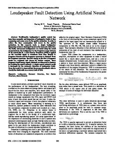
Vibration data was collected at NASA LeA is Research (,enter as part of a joint NASA/Navy/Army Advanced Lubricants Program to reflect the effect of various faults in an 01-58A main rotor transmission (Lewicki et al., 19A92). The configuration of the transmission which was tested in the NASA 500-hp Helicopter Transmission Test Stand is shown in Fig. 1. The vibration signals were measured by eight piezoelectric accelerometers (frequency range of up to 10 KhIz), and an FM tape recorder was used to record the signals periodically once every hour, for about one to two minutes per recording (at the tape speed of 30 in/sec, providing a bandwidth of 20 KlIz). Two chip detectors were also mounted inside the transmission to detect the residues caused by component failures. The location and orientation of the accelerometers are shown in Fig. 2, and the schematic of the vibration recording/monitoring system is shown in Fig. 3. In these experiments, failures occurred naturally. The transmission was run under a constant load and was disassembled/checked periodically or when one of tile chip detectors indicated a failure. A total of five tests were performed, where each test was run between nine to fifteen days for approximately four to eight hours a day. Among the eight failures occurred durini,, thiese tests (see Table i),

therp w,,r,, th

;'oe,

nf l:•

bt.iin'• f:.ii rc, t-ree cases o" -"m

Planet Bearing

Mast Ball Bearing

Planet Gear Ring Gear

Spiral Bevel Gear Cpiral Bevel Pinion

Sun Gear

Triplex Bearing

Gear Roller Bearing Mast Roller Bearing

Pinion Roller Bearing

Duplex Bearing Figure 1.- Configuration of the OH-58A main rotor transmission.

gear failure, two cases of top housing cover crack, and one case each of spiral bevel pinion, mast bearing, and planet gear failure. Insofar as fault detection during these tests, the chip detectors were reliable in detecting failures in which a significant amount of debris was generated, such as the planet bearing failures and one sun gear failure. The remaining failures were detected during routine disassembly and inspection. Vibration monitoring during testing was not used as a diagnostic tool.

3

SIGNAL PROCESSING

In order to identify the effect of faults on the vibration data, the vibration signals obtained from the five tests were digitized and processed by a commercially available diagnostic ana-

4

#1, 2, 3 attached to block on right trunnion mount #4. 6, 7, 8 studded Vi housing through steel inserts #5 attached to block on input housing

Left trunnion mount

0A Transverse

0

0

.4

e

Longitudinal

Right trunnion mount Transmission output

St Transmission input

w.

Figure 2.-LocatIon of the accelerometers on the test stand.

5

Vertical

Longitudinal

Output Accelerometers

Input OH-58A Transmission

Charge Amplifiers

Attenuators

VU Scopes

FM Tape Recorder Figure 3.-Schematic of vibration recording/monitoring.

lyzer (Stewart Hughes Limited, 1986).

Three processing modules of the analyzer were used:

1) Statistical Analy.sis (S'At7. 2) B!ascband Power Spectrum Analysis (BBPS), and 3) TBcaring Analysis (BRGA). For analysis purposes, only one data record per day was used for each test. These data records were taken at the beginning of the day unless a fault was reported. which in that case, the record taken right before the fault incident was selected to ensure that the data record reflected the fault. Also, in order to reduce estimation errors, each data record was partitioned into sixteen segments and parameters were estimated for each segment and averaged over

these segments. The data records as well as the parameters obtained from the above processing modules were then transferred to a personal computer for further analysis. The schematic of the data acquisition apparatus and the parameters obtained from each module of the diagnostic analyzer are illustrated in Fig. 4. Note that the objective of this paper is to demonstrate the MVIM pattern classification scheme, not to develop/verify individual diagnostic algorithmis. The algorithms descrilbod in the next subsections were used to determine inputs to the MVIM method, but may not be optimnized for transmission health imonitoring.

'l~rest 1f

#

N7umiber of

T

9 9

jaiu I)yri-s Sun gear tooth piit S pi ral 1)ev(l plinion- scornitu g/ ha%v None Plaiiet beariig #2 inner race sp:ll

Micropitting Oilmsn

4

1.5

5

11

tail

Planet bearing #3 in ner race spal I

'N

i

i

Sun gear tooth pit______

________________________Top

Suin gear teeth spalls Planet gear tooth spail housing cover crack

Table 1: Faults occurred (luring the exp~erimlents.

3.1

Statistical Analysis

It is general-ly believed tha.ý th- probability density, fun ction (p).d 4.) of the vib ration amnplituide is near Gaussian when iniachinerv is heal thy, and that Its shape chang-es when a dlefect appearsý. The Statistical Analysis Modulc of the (liagnostic analyzer estimates p~aramueters that would characterize such change.

Among die Jparaiiieters available from this mod ule, the skewness.

kurtosis, crest factor, and peak-to-peak value of vibration data are reported to be gpod indicators of localized dlefects in rotating mnachinery (e.g,. set- Dyer andl Stewart. 1978). A brief descriptionl of these p~aramieters is as follows:

"* Skewness Coefficient. The skewness coefficienlt

T.jreprsents

thlt SVnInI)TrV Ofpraily

densi tv, function of the vibration ampli1tu de. Siince the skewness cudfit cirt of a (.a st aisiM distri hut ioa is zero, any deviations of the skewness coefli1cient from zero Canl be duiie to

"* Kurtosis Value. The, kutrtosi.s, value. which repre-sents the concentration of heights arounld

the mean linoi of thie p robabhility dlensity fuintction, is equiial to 31for a C aussian (list ri butiOnl

As such, k iiirtosis ValueS lAr'ger tt alt 3 are reportedl to be ind(icat ors Of luca hi17041 defects ( D.) tr

and Stewart. 1978).

"* Crest Factor. Similar to the kurtosis value, the rest factor is u=ed

th

dswnhe, the

'peakness' of tew t rolaabilkty density funmtion (Braun, 190(). llowever. urnlike the, kurt,, value, the crest factor is only a relative, nweasure. .Moreover., sinir

the c rest fa to r i• fwr,;

likely to be a~fected by a single outlier, it is generadly not as robust as thli kurtt

e•

.l

w

"*Peak-to-Peak Value. When failures occur, the amplitude of the vibration ten td to increase in both upward and downward directions and thus the peak-to-peak valu,, is

expected to increase.

The above statistical paramrrt, rs were obtained for the five tests. The results indicate that ione of the parameters provide' a good ir~idictiin of all the faults

1-or example, the aver;,oged

kurtosis values (if the vibration signals fromu the eight accelerometers are shown in Fig. 5 for the five tests. The results indicate that the kurtisis value reflect: only the fault incident at the end of Test #5,

and that it is not sensitive to the other six fault incidents in the Lther tUots (tarked

by asterisks). The significant increase in the kurtosis value at the enm caused by the severity of faults in this tst housing crack).

of Test #5

is perhaps

(i.e., sun gear teeth spall. planet tooth spall. and top

OH-58A Main Rotor Transmission Vibration Signals FM Tape Recorder

Digitization/Processing

STAT

(1) Skewness (2) Kurtosis (3) Crest Factor (4) Peak-to-Peak

BSPS

(5) RMS (6) WHT (7) RFR (8) TEO-G (9) TEO-P (10) TM1-G (11) TMI-P (12) CEP(1911)

BRGA

(16) (17) (18) (19)

BE BKV EB ET

(13) CEP(572)

(14) TON(1911) (15) TON(572) Figure 4.-Schematic of the data acqutsitloir a'.paratus. as well as the parameters obtained froer the diagnostic analyzer.

4.0

,

-I-I,

Test 01

Test #2

Test #3

rest #5

Test #4

3.8

3.4

._

0

S3.2

3

3.0 2.8 2.6 0

10

40 20 30 Sample Data Points, N

50

60

Figure 5.-Averaged kurtosis values for the five tests from the Statistical Analysis Module. Faults are indicated by asterisks.

3.2

Baseband Power Spectrum Analysis

Spectrumn analysis (or frequency domain analysis) is perhaps the most widely used technique in vibration signal processing, as failures such as unbalance, misalignment, wear, and roller bearing spadling produce a clear change in the spectrum (e.g., see Dewell and Mitchell, 1984; Randall, 1982; Taylor, 19S0: Lees and Pandev, 19801,

However, in complex machinery whore

the background noise masks the basic distress signal, changes in the spectra cannot be easily lBas distinguished (Pratt, 1986). The

cband Power Sprctlrurn Analysis Module provides sever-d

parameters that can be ai>,ociated with the frequencies generated iw individual components of the transmission. The parameters obtained from this module are:

I

I)

* Root-Mean-Sq

u a

re.

The root-uiatn-.,quare ( UiMS) value of the vibration am plitli Ii

represents the overall energy level of vibrations. As such, the It NS val,,e can b, i,-,,Id to detect major changes in the vibration level. SWXhite Spectrum. The white spectrum (WHT) represents the rins level of the sign;d minus its strong tones. Therefore, it denotes the energy level in the base of the spectrum. Since certain failures, like wear, do not seeni to increase the strong tones created by shaft rotation and gear mesh, the energy in the base of the spectrum could potentially be a powerful detection paraineter for wear-related failures. * Rice Frequency. The rice frequency (RFR) denotes the position of the 'center of gravity' of the spectrum. Therefore, it can reflect any major changes in the shape of the spectrum 'hat may have been caused by faults. * Comparison Analysis.

Failures in rotating machinery tend to increase spectral lev-

els. The Coinparison Analysis Function provides several statistical parameters about the spectral ratio between the current spectrum and a baseline spectrum. The baseline spectrum could either be the spectrum of vibration at the beginning of the test (TEO) or the spectrumn of vibration from the previous record (TMI). Among the statistical parameters obtained from this function, TEO-G and TEe-P, which denote the energy level (rms) and the mean value, respectively, of the spectral ratio with respect to the first spectrum, and T=M 1-(

and T"IM I- , which represent the energy level ( rms) and the mean value, re-

spctively, of the spectral ratio with respect to the preceding spectrum. are particularly effective in representing differences between the current and the baseline spectrum. * Metr- -pstral Analysis.

The Mc1acepstrurn

Analysis Function is used to detect the

periodic featriies of the vibration signal (Lyon and Ordubadi, 1982; (hil(ders

et al.. 1977).

The piaraint,ters obtained fromi t1 is funiction are measures of the energy level at a given freqluency and it• harmnonics.

The two frequencies selected for this analysis were the

Il

toothlnes

It1g frequency of the spiral bevelI mnesh (1911 l1z) anld the toJotlIlleI'sIlIlIg

of the planetary inesh

f 1 ie4III"I(v

5'72 liz). The parameters calculated for thes*e two fresqueon'Ois a4,

represented as CEP(1911) and CEP(572). e Tone Analysis. The energy level associated with a particular tonel

within a spjtrum

is also a good indicator of faults. Various faults like uibalance and iuisalign9Tinet tnid to increase the tone energy. The two parameters ToN(o1911) and TON(572) obtained for this analysis represent the tone energies at 1911 Hz and 572 liz, respectively.

The above parameters from the Bascband Powcr Spectrum A nalysis Module were computed for the five tests. The results indicate that although some of these parameters are good indicators of specific faults, they are also prone to false alarms. For example, the averaged TM 1-G values of the vibration signals, from the eight accelerometers, obtained for the five tests are shown in Fig. 6. The results indicate that while this parameter is sensitive to one of the faults in Test #3 (i.e., the first fault caused by planet bearing inner race spall), it also contains a spike on day 5 of Test #1 which could result in a false alarm.

3.3

Bearing Analysis

The vibration energy of bearing elements is usually lower than those produced by gears, shafts. and sometimes noise. As such, bearing faults cannot be readily detected through abnormalities in the bearing tone. However, since bearing faults such as spalling produce time domain impulses which modulate the bearing shaft frequency over a wide range of frequencies, there are features of high frequency vibration that would reflect such bearing faults (Mathew and Alfredson. 19,,4: Braun and Datner, 1979). The 11caring Analysis Module is designed to extract such features. This module uses a hotcrodyncr to demodulate the vibration signals and obtain an amplitude envelope (e.g., see Courrech ,lnd Gaudet, 1985), and then calculates the power spectrum of this envelope (i.e., spectral envelope) so that its various features (parameters) can be estimated for

12

Test #1 Test #2

Test 03

Test #4

Test #5

1.6 1.4

S1.2 4)

~1.0 0. S0.8 0.6 0.4

0.2

0

10

20 30 40 Sample Data Points, N

50

60

Figure 6.-Averaged TMI-G valuea for the five tests obtained from the Base-band Power Spectrum Analysis Module. Faults are indicated by asterisks. bearing fault detection (Dyer and Stewart, 1978; Yhliand and Johansson, 1970). The parameters obtained from this module are:

"• Envelope

Band Energy. The band energy (BE), which is calculated as the sum of the

mean and standard deviation of the full bandwidth envelope, represents the overall energy level of the envelope. This parameter is expected to be sensitive to most bearing faults which increase the level of vibration.

"* Envelope

Kurtosis Value. The kurtosis value of the envelope (BKV) is estimated to

reflect imni)ulsive behavior of vibrations produced by localized bearing faults.

"* Envelope

Base Energy. The envelope base energy (EB) represents the base energy of

the spectrum after all tones have been removed.

13

This parameter is expected to reflect

heavy bearing dlamage. e Envelope Tone Energy. The tone energy (ET) represents the total energy winus the base energy. This parameter is expected to reflect localized bearing faults. The above parameters from the Bearing Analysis Module were computed for the five tests. The results indicate that most of the parameters are not very sensitive to the faults occurred during the tests. For example, the averaged values of the kurtosis value of the envelope (BKV) are shown in Fig. 7. The results indicate that while the BKV is relatively sensitive to the faults in Tests #I and #3, it exhibits a spike in Test #3 which could potentially result in a false alarm.

5.5

Test #1 Test #2

Test #3

Test 94

Test #5

5.0

>

4.5-

Oil

InI

W1

CO

•

4.0-

3.630'

0

10

20 30 40 Sample Data Points, N

50

60

Figure 7.-Averaged BKV values of the envelope kurtosls values for five tests. Faults are Indicated by asterisks.

14

4

THE MVIM METHOD

The MVIM method is based on a multi-valucd in•lucnc, matrix (NIVIM) which represoiits the uncertain relationship between various faults and ineasureinents (Danai and Chin, 1991). Measurements in this method are monitored in-process and converted to binary nunbers through flagging (see Fig. 8), which are posted in a vector of 'flagged measurements'. Flagging in this

method is performed by a quantization matrix, and detection is performed by matching this vector of flagged measurements against the individual columns of the influence matrix (influence vectors). Influence vectors which represent the no-fault signature and the fault signature are continuously updated by a learning algorithm to improve detection.

Sensory Data

Processed Measurements

Processing

Binary Measurements

Flagging

Estimated Fault Vector

MVIM

Figure 8.-4etection strategy Inthe MVIM method.

4.1

Detection Model

The multi-valued influence matrix A representing the no-fault signature and fault signaturc is defined as Y(t)

A

X(t)(1

to relate the flagged mcasuremrent vcctor Y(t):

Y(t)

{y,(t), Y2(t), ...

15

,

y,,(t)}T

(2)

to the fault vector X(t): X(t) = {XI(t), where 7n is the number of measurements.

)T }r(

1

In the above equations, the vectors Y and X arc

binary vectors; i.e., the yi (individual flagged measurements) and xi (the no-fault variablel and the fault variable

X2)

x,

can only be equal to 0 or 1, representing the status of the particular

measurement and fault at the time, respectively. Note that the the components of the (in x 2) influence matrix A in Eq. (1), which represents a functional mapping between Y and X, are between 0 and 1 defining the causal relationship between individual flagged measurements yi and the no-fault and fault cases. For example, an a 12

=

0.8 implies that the possibility of the

1st measurement being flagged at the instance of fault is 0.8, or an a31

=

0.2 indicates that a

0.2 possibility exists that the 3rd measurement is flagged for a no-fault case.

4.2

Detection

Detection in the MVIM method is based on matching the vector of flagged measurements against the individual influence vectors. The closeness of vectors in the MVIM method is based on their orientation. Accordingly, the possibility of occurrence (diagnostic certainty measure) of the nofault or fault case is defined as the cosine of the angle between the corresponding influence vector and the vector of flagged measurements. The geometric representation of this reasoning, for a three dimninsional measurement vector (n = 3), is illustrated in Fig. 9. Vectors V1 and V2 in this figure represent the influence vectors associated with the no-fault and fault case, respectively, and vector Y denotes the vector of flagged measurements. In the MVIM method, the vector of diagnostic certainty measures which ranks the variables x, and x 2 for their possibility of occurrence is defined as

cosS=

=

Z2

~

COSQ a2

VT=

(4)

2

where at and (k.2 denote the angles between the influence vectors V 1 and V 2 , respectively, and

16

Y(t)

Figure 9.--Geometrc representation of diagnostic reasoning In the MVIM method for a three dimensional case.

the flagged measurement vector Y, and Vj

(j = 1,2) and Y are the normalized forms of vectors

Vj and Y, respectively, defined as

V

{--

=v -}(5)

an (1

Yi = II - -,

Detection in the MVITN method is based on obtaining the vector of diagnostic certainty mea-sures X. To obtain X, however, the normalized form of the influence mnatrix, A,

A=V

1

V2 ]

is requiiired. Since this matrix is not known a priori, it will have to be estimated.

17

4.3

Estimation of A

One of the main features of the MVIM method is its capability to use the detoction ,error as feedback in estimating/updating A. Based on this learning strategy, individual colu nin of tOe influence matrix are adjusted recursively after the occurrence of fault, or when a flag is posted in a no-fault case, to minimize the sum of the squared detection error. The estimation algorithm of A which is based on recursive least-squares estimation (Ljung, 1987) is given in (I)anai an(d Chin, 1991), where its performance is demonstrated in simulation.

4.4

Flagging

In the MVIM detection system, flagging of measurements is performed by a quantization matrix. For flagging, the measurements P are multiplied by the weights of the quantization matrir Q

Q

[W1

w, ...

...

W"J

,

(7)

and hard-limited as

f1 Yi=

0

when pTW; > 0.5 otherwise

(8)

to produce the binary vector of flagged measurements Y (see Fig. 10). This vector is used for both detection, as well as estimating/updating the MVIM. The vectors Wi in Eqs. (7) and (8) represent the columns of the quantization matrix associated with individual measurements. The vectors of the MVIM are trained based on the flagged measurements y, (see Eq. (8)). Therefore, they are directly influenced by the flagging operation. In order to improve the flagging operation, the quantization matrix is adapted during a training session. Ideally, we would like the magnitude of all flagged measurements yi to be equal to 0 for no-fault cases and I at fault instances. Therefore, the components of the quantization matrix are adjusted to produce such ideal flagged measurement vectors (see Fig. 10). The proposed quantization matrix uses a sample set of measurement-fault vectors to tune

18

Flagging Sensory Data

SSignal

1

S yeEstimated Bihary Fault Measurements Vector

Prdcessed M~asurements

-- X---

Quantization L-"

P

Processing

Matrix

|MVIM S Limiter: Y

*

V

l

Target

Sx Figure 1O.-Schematic diagram of adaptation In the MVIM method.

its parameters iteratively. For this purpose, it uses recursive last-squares adaptation to minimize the sum of square errors between the individual flagged measurements produced by the

quantization mutrix and their ideal values. This learning algorithm has the form w~ij(iz,) = w~j(fi - 1) + 1I(PI - 1) [(•)-PT(,4)'w,(tt - 1)]

(9)

where the wjj denote the components of the quaritization matrix, ýL is the iteration step, ýi represent the ideal value of flagged measurements (i.e., yi = 1 for fault cases, and ýi = 0 for no-fault cases), and the lj denote the comlponents of the adaptation gain vector L, updated according to the relationship (Ljung, 1987)

R(+i - 1 )PT'(JL) I + P(ji)R(P( - 1)PT( p) 1

where matrix R denotes the covariance matrix in least-squares estimation computed as

R(tp) = R(It - 1) - L(9)P(i)R(p - I

19

(10)

5

DETECTION RESULTS

The averaged values of the nineteen parameters obtained from the diagnostic analyzer were used as the components of the measurement vector P to train and test the MVIM (see Figs. .4 and 10). For scaling purposes, each parameter value was normalized with respect to the value of the parameter on the first dlay of each test. As explained in the previous section, the MVIM method requires a set of measurements during normal operation and at fault incidents to estimate the no-fault and fault signatures. Since in the experiments the exact time of fault was not known, the time of fault occurrence was conservatively set on the last day, or right before failure was verified through disasselubly. Similarly, no-fault cases were assumed only for the first day of each test, and after faulty coinponents were replaced. The specification of vibration data as fault and no-fault on various days of each test are listed in Table 2. For Tests #1 and #5, only the data from the last day (day 9 and day 11, respectively) was associated with a fault case, since faults in these tests were only found on the last day during routine disassembly. For Test #2,

the data from all of the nine

days were marked as no-fault, since no faults were detected during inspection at the end of the ninth days. For Test #3, the data from days 1, 5, and 10 were associated with a no-fault case, because they were obtained directly after faulty components were replaced on days 4, 9, and 13.

For Test #4,

data from days 1-8 was attributed to a no-fault case, since no faults were

detected upon inspection at the end of the eighth day. For this test, the data from days 12 and 15, which were collected before faulty conlponents were replaced, were associated with fault incidents. Note that the data from (lay 13, obtained directly after the replacement of the faulty component, is also associated with a no-fault case. The effectiveness of the MVIIM detectionl method was evaluated with different training sets.

20

Day I

2 3 4

Test # I no-fault -

-

5

6 7 8 9

10

-

fault

Fault Status Test #2 flst #3 Test #4 no-fault no-fault no-fault

no-fault no-fault no-fault

fault

no-fault no-fault no-fault

no-fault Ino-fault

no-fault

no-fault no-fault no-fault no-fault

no-fault no-fault no-fault no-fault

fault

no-fault

11 I 12 13 14 15

'Wt #5 no-fault

fault fault

fault no-fault fault

Table 2: Association of data from each day of the 5 tests with fault and no-fault cases. The mark '-' denotes that data from that day cannot be specified.

For this purpose, training sets were formed based on parameters from various combinations of five tests (see Table 3). For each training case, the initial values of the MVIM (19x2) and the quantization matrix (19x 19) were set to 0 and I, respectively, and training was continued until perfect detection was achieved in the training set (i.e., no false alarm or undetected fault was found in the training set). The MVIM was then tested on all the data from all of the five tests. Performance of the NIVIM was represented by the total number of false alarms and undetected faults it produced during testing (denoted as Total Test Errors in Table 3). The detection results produced by the NIVIM for 30 different cases of training are shown in Table 3. For comparison purposes, the results obtained from the NIVINI are contrasted against the results obtained from a multi-layer neural net (e.g., see Hertz et al., 1991; Rumelhart et aL.. 1988) which was trained and tested under the same conditions.

The neural net was trained

with the back-lpropagation learning algorithim and contained 40 hidden units. This number of hidden units was selected within a range of 30 to 50 hidden units to optimize its generalization

"21

ab~ili ty. For tt~in~iiig

the not, the learninig rate and~ momcien tum i cooli cient were, ,vt at 0.2 ani

0.8, respectively. The above paramefters were selected within a range of 0.2 to U.S through trial and error so as to op~timhize the convergence speed of the net. The results in Tab)le :3 indicate that the INI VIM was able to provide perfect detection

when

faults were fully represented by the tra~ininigsets (i.e., Cases #18, #21. #24, #25, #28, #29. and #30), and that it produced better results th mnthe neural net in most of the cases. SpecificallY.

the INIVIM produced better results in nineteen of the test cases, produced identical resulits InI ten cases, anl wvas outperformied in only one case. Upon a casual inspection of the training et s that enabled MNVIM to perform perfect (detection, it can be observed that Tests #3 and] #1I are includIed in all of them. This implies that the MVIMN needs the parameters from1 these two tests to establish an effective pair of signatures for no-fault and fault cases. Note that without Test #3, the MVIM p~rodulces one undletectedl fault andl one false alarm (Case #27). and( without le~st

#4 it produces one undetected fault (Case #28). Note that the multi-layer neural net cou'd niot provide perfect detection even when trainedl with all of the five tests (Case #30).

22

]'I)

2

3

3

I

Neural Net IVIM N, araNNet[1

-

1 1

5

1,2

6

1.3

1,4 8

1.5

9

2,3

1

2.4

i

.l

0 3

I'VIN '\12 Neural Net MVIM

4

i

Li

1

13

4 "2

1 3

6 2

Neural Not MNVIMI2 Neural Net MVIM

4

0t

Neural Net MVIM Neural Net MVIM Neural Net

1 1 1 1 1

1 1 2 2 1

2 2 3 3 2

IMVIM Neural Net N'I\"IN

I , ;3

1 2 1

2 3 ,

12

1 2

-4 3

2 0

I

_2

11

2,5

Noural Net

3

"2

5

_NIVII

12

3.4

Neua a Net M\I.\ Neural Net

3 2 0 0

2 2 0 3

5 . 0 3

1

0

1,

r

_______M\VIN

1.1

4.

15

1,2,3

Neural Net MVIM Neural Net

16

1,2,4

Neural Net

3 1 1 2 2 2 1 1_

MVIM __MVIINI

17

1,2,5

iIS

1,3.11

P0

1,3,. 201,1,

Neural Net MVIM Neural Net1 MVIIM

1 2 0 1 IF_ 2 2

0 0

N(eural Net 1V I\I (' rd Net

0 2 1

IVI.I

__1

23

T I

~

1

3 '2 3 2 3

3 3 3

0

1 0

() 1

3 2 '2 2

fJCase # Ij

Frainling I Diagnostic Dta sets

%lethlod

2,3.4-

Neural Net %MVIIM Neural Net

________I

21 22

2.3,5 ____INI __

_

__

2:3

2.-4,5

24

3:14.5

25

1.2,3.4

26

_

(

unidetectedi-

VI % Neural Net %VI vI% Neural Net

Fal

ze

Faults

Alarmls

2 0 1

02 0 2

1

0

:3

1

'st

0 :3 -1

VI'%

1 02

4

__-

1 2

EFrror:-,

2

0

0

0

1,2.3,5

Neural Net MIN M %1 Neural Net

2 () 2

0 0 1

2 0 :3

27

1,2,4,5

Neural Net

1

1

2

28

1,3,4,ý5

Neur~ai -et

1I

29

2,3,4,5

Neural Net

2

0

30

1.2,3,4.5

Neural Net

1

0

______

-

-,

1

2 1

Table 3: Detection results obtained from NI\VIMI and] a multi-layer neural net w.hen trained with dlifferent dlata set~s.

6

MEASUREMENT SELECTION

The %IVIM method cani also assess the significance of individual parameters in detection.

It

is generally assum~led that the parameters whiichi reflect the faults more effectively facilitate training, p~articullarly wh~en the success of training is based upon detection capability within the training s,-t.

Threw(fore, whol en udi viduial parameters are d1iscarded

(letectabl~jity must be reflected in the t.rainmming timie for that set.

,

their influence on overall

Thiis means that when anr

'imp~ortant' parameter (measurement) is dliscarded from thle training Set, for the faults are to be cliaracte rized by thle romiram ining paramiieters ( meas ure men ts ), the tralininig will be more difficuli t aLn(I, thus, umore timue-consli iiiirig.

2.1

Ili IIrdel

wais selected.

I t,-. t the d)(we I l A\mmi

i, I aI

thit, varimi,

;1111111

triitilmig " •twt

"whichI Col tai ned the si II'l lest num i ber of data

't

1I' k. perf ct

l p1

W

in Table 3 satisfviyra

set

d-tect i

this, condi tiota

r ni

(';'.-

IIttl

12

(i.e., Tests g 3 and #4) " as solIected. In d(ivid u ;l

parameters were tlen (1ti.cardod mric at a tOine from this trraining s.ct ti fortm new reducid s-,ts for training the M\"I M The number of training epochs' required for each reduced set is shown

in Table .1, with the discarded l)araineters imposing higher than 9 epochs (obtained for the full set) marked by a plus sign.

[

Case # 12 (Test # 3 and #4) fiPara'eter D~iscarde

I

j

_

,Number of Training Epochs

Undetected Faults

False Alarms

9

0 0 0 00 0

0 0 0

0

0

9

0

0

9

0

9

o

9

0

0

None #i 1 #2 3+ #_ _ 5

I

#__ #7_0

9 9 25 9 9

0

0

#9 #10

# II+

0

T -o

10

0

0...{

#12#13+ #1,1+

100" 11

0 0 00

5 0 0

# 15+ #l1+ #17+

37 10 "22

0 0 0

0 0 2

#

# is8

00

199

0

0

Table -1: The elfect of diPa rded paramneters on training tirae aind test results. The particullar sets that required a longer training time than the full set are zitarked by '+'. The '*' denotes that fulIl detection within the training set WaS nlever acthieved. ilasss through the training set

225

Based on the results in Tahle 4, the elimiiiination of Parameters #3 (crt P), #12

(CEP(1911)), #1:3

(CEP(:S72)), #1.1

f;t, tor). #' 1 (I

M1I

(TON(1911)), #1V) (TONV!>72)), # 16 (111), ;-,id

#17 (1BKV) from the training set adversely affected training. This (-u'd imply that th,-,, ,it parameters are particularly important in characterizing the signaturs for the no fault and fult case, and that Parameter #12,

whose elimination jeopardized training, is critical. liv thie sa1m,1

analogy, the results in Table 4 indicate that discarding Parameters #7 and #

IS

may bIe ven

beneficial to training of MVIM. In order to validate the above findings. various combinations of parameters from ',ests #3 and #4

were grouped into training subsets. Training started with th, smallest poi1

which included only two parameters.

sul,,t l,'

As the MVIM did not converge with this subset, tOw

subset was expanded further until successful training was obtained for the M\VINI. The first subset that resulted in perfect training for the NIVIM was one with twelve parameters, of which eight parameters were those that were identified as 'important' before (i.e., Parameters #3, #111. #12,

#13,

#14,

#15,

#16,

and #17).

In fact, through further analysis it was ascertained that

the smallest subset of parameters that would provide perfect training for the INIVIMI consikts of these eight parameters, and +hat discarding or replacing any of these eight parameters results in a non-trainable situation. Addition of more parameters Lo this subset did not make a difference. The same type of analysis performed with the NIVIM method could potentially be performed with a neural net. However, neural nets provide different detection results with different number of hidden units. As such, for each number of inputs (parameters) the optimal number of hidden units need to be selected, which would then affect the number of epochs required for training. This will complicate the criteria for measurement selection of the type descril)ed above. The advantage of the NIVINI method over a neural net is that its structure is fixed based on the number of its inputs, and thus the number of training epochs would directly reflect the significance of individual measurements.

26

7

CONCLUSION

Fault detection of helicopter power transmissions through pattern classification is deinonstrated. For this purpose, the M VIM detection method is used to construct no-fauilt and fault signaturem based on vibration data reflecting the effect of various faults in an 01-58A main rotor transmission. Implementation results indicate that the MVIM can provide perfect detection when the full range of fault effects are extracted through appropriate signal processing. The M\VIM method can also assess the significance of individual measurements. Based on this assessment, it is shown that an optimal subset of measurements can be selected so as to reduce processing time for in-flight implementation purposes.

ACKNOWLEDGEMENTS The authors would like to express their gratitude to Sikorsky Aircraft Company for its continued support of this project and NASA for providing the experimental data. This work was supported in part by the National Science Foundation (Grants No. MSS-9102 149).

27

DDNI-90156.14 and

REFERENCES Astridge, D.C.: Vibration Health Monitoring of the Westland 30 Helicopter Transmission- .. )evelopment and Service Experience. Detection, Diagnosis, and Prognosis of Rotating Machinery to Improve Reliability, Maintainability, and Readiness through the Application of New and Innovative Techniques, T.R. Shives and L.J. Mertaugh, eds., Cambridge University Press, New York, 1988, pp. 200-215. Braun, S.: Mechanical Signature Analysis-Theory and Applications. Academic Press, New York, 1986. Braun, S.; and Datner, B.: Analysis of Roller/Ball Bearing Vibrations. Mech. Des., vol. 101, Jan. 1979, pp. 118-125. Cempel, C.: Vibroacoustical Diagnostics of Machinery: An Outline. Mech. Syst. Signal Proces., voi. 2, no. 2, 1988, pp. 135-151. Childers, D.G.; Skinner, D.P.; and Kemerait, R.C.: The Cepstrum: A Goide to Processing. Proc. IEEE, vol. 65, no. 10, Oct. 1977, pp. 1428-1443. Chin, H.; and Danai, K.: Fault Diagnosis of Helicopter Power Trains. Proceedings of the 17th Annual National Science Foundation Grantees Conference in Design and Manufacturing Systems Research, Society of Manufacturing Engineers, Dearborn, MI, 1991, pp. 787-790. Chow, E.Y.; and Wijisky, A.S.: Analytical Redundancy and the Design of Robust Failure Detection Systerts. IEEE Trans. Autom. Control, vol. AC-29, no. 7, July 1984, pp. 603-614. Collier-March, A.: Operational Experience with the Advanced Transmission Health Monitoring Techniques on the Westland 30 Helicopter. Presented at the 11th European Rotorcraft Forum, 1985, Paper 43. Courrech, J.; and Gaudet, M.: Envelope Analysis-the Key to Rolling-Element Bearing Diagnosis. Bruel & Kjaer Application Notes, a Pamphlet, Larcenk & Sons, Denmark, 1985. Danai, K.; and Chin, H.: Fault Diagnosis with Process Uncertainty. J. Dyn. Syst. Measur. Control, vol. 113, no. 3, Sept. 1991, pp. 339-343. Dewell, D.L.; and Mitchell, L.D.: Detection of a Misaligned Disk Coupling Using Spectrum Analysis. J. Vib. Acoust. Stress Reliab. Design, vol. 106, Jan. 1984, pp. 9-16. Dyer, D.; and Stewart, R.M.: Detection of Rolling Element Bearing Damage by Statistical Vibration Analysis. J. Mech. Des., vol. 100, Apr. 1978, pp. 229-235. Hertz, J.; Krogh, A.; and Palmer, R.G.: Introduction to the Theory of Neural Computation. AddisonWesley, Redwood City, CA, 1991. Kaufman, A.B.: Measure Machinery Vibration-It Can Help You Anticipate and Prevent Failure. Instrum. Control Syst., vol. 48, Feb. 1975, pp. 59-62.

28

Lees, A.W.; and Pandey, P.C.: Vibration Spectra from Gear Drives. Second International Conference on Vibration in Rotating Machinery, Mechanical Engineering Publications, london, U K, 1980, pp. 103-108. Lewicki, D.G.; Decker, H.J.; and Shimski, J.T.: Full-Scale Transmission Testing to Evaluate Advanced Lubricants. NASA TM-105668, 1992. Ljung, L.: System Identification: Theory for the User. Prentice-Hall, Inc., Englewood Cliffs, NJ, 1987. Lyon, R.H.; and Ordubadi, A.: Use of Cepstra in Acoustical Signal Analysis. J. Mech. Des., vol. 104, Apr. 19S2, pp. 303-306. Mathew, J.; and Alfredson, R.J.: The Condition Monitoring of Rolling Element Bearings Using Vibration Analysis. J. Vib. Acoust. Stress Reliab. Des., vol. 106, July 1984, pp. 447-453. McFadden, P.D.; and Smith, J.D.: A Signal Processing Technique for Detecting Local Defects in a Gear From the Signal Average of the Vibration. Proc. Inst. Mech. Eng., vol. 199, no. C4, 1985, pp. 287-292. Mertaugh, L.J.: Evaluation of Vibration Analysis Techniques for the Detection of Gear and Bearing Faults in -Helicopter Gearboxes. Detection, Diagnosis, and Prognosis of Rotating Machinery to Improve Reliability, Maintainability, and Readiness through the Application of New and Innovative Techniques, T.R. Shives and L.J. Mertaugh, eds., Cambridge University Press, New York, 1988, pp. 28-30. Pau, L.F.: An Adaptive Signal Classification Procedure Application to Aircraft Engine Condition Monitoring. Pattern Recog., vol. 9, 1977, pp. 121-130. Pratt, J.L.: Engine and Transmission Monitoring-A Summary Promising Approaches. Detection, Diagnosis, and Prognosis of Rotating Machinery to Improve Reliability, Maintainability, and Readiness through the Application of New and Innovative Techniques, T.R. Shives and L.J. Mertaugh, eds., Cambridge University Press, New York, 1988, pp. 229-236. Randall, R.B.: A New Method of Modeling Gear Faults. J. Mech. Des., vol. 104, Apr. 1982, pp. 259-267. Rumelhart, D.E.; Hinton, G.E.; and Williams, R.J.: Learning Error Representation by Error Propagation. Parallel Distributed Processing--Explorations in the Microstructure of Cognition, Vol. 1: The Foundations, D.E. Rumelhart and J.L. McClelland, eds., MIT Press, Cambridge, MA, 1988. MSDA User's Guide. Stewart Hughes Limited, Southampton, UK, 1986. Taylor, J.I.: Identification of Bearing Defects by Spectral Analysis. J. Mech. Des., vol. 102, Apr. 1980, pp. 199--204. Yhland, E.; and Johansson, L.: Analysis of Bearing Vibration. Aircr. Eng., vol. 42, Dec. 1970, pp. 18-20.

29