Fault detection of the boiler unit using state space

Fault detection of the boiler unit using state space neural networks A. Czajkowski ∗ K. Patan ∗,1 ∗ Institute of Control and Computation Engineering, University of Zielona G´ ora, ul. Podg´ orna 50, 65-246 Zielona G´ ora, e-mail: {A.Czajkowski, K.Patan}@issi.uz.zgora.pl

Abstract: This paper deals with the application of state space neural network models to fault detection of the boiler unit. The work describes problems such us selecting the proper threshold for compromising both fault sensitivity and early fault detection, designing proper neural network structure or calculating performance indexes. All the simulation data used in experiments are collected from the simulator of the boiler unit implemented in Matlab/Simulink. Keywords: state space model, dynamic system, neural network, fault detection. 2. BOILER UNIT

1. INTRODUCTION Recently, it has been observed an increasing development of the Fault Diagnosis (FD) methods for the Fault Tolerant Control (FTC) system desing purposes. It is straightly connected to the advantages of the systems which can maintain current performance as close to the desirable one, and preserve stability conditions in the presence of faults. Faults and equipment failures directly affect the performance of the control system and can result in large ecomomic losses and violation of the safety regulations. During the fault tolerant control system design, the basic problem is the early detection and identification of possible faults. The main objective here is to use approaches providing the acceptable behaviour of the control system in the case of a critical fault and to shutdown the system safely. The paper focuses on the first stage of FTC system design which is the modelling of the system. In this work to construct the model of the system the so called State Space Neural Networks (SSNN) are applied. The SSNN model is then used to carry out the fault detection by analysing the residual. The state space model estimates the state vector of the system and in cases when states of the system are measurably available residuals can be calculated as differences between states and their estimates. The methodology presented in the paper is tested on the example of a boiler unit. The paper is organized as follows. Section 2 presents a general desciption of the boiler unit and provides information about faulty scenarios considered. The state space neural networks are described in Section 3. Section 4 presents a fault detection algorithm, while experimental results are included in Section 5.

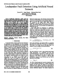
The object considered in this work is the laboratory installation developed at the Institute of Automatic Control and Robotics of the Warsaw University of Technology. The installation is dedicated for the investigation of diagnostic methods of industrial actuators and sensors Koj et al. (2005). The whole system consists of the boiler, storage tank, control valve with positioner, pump and transducers to measure process variables. The boiler is realized in the form of a horizontally placed cylinder, which introduces a strong nonlinearity into the static characteristic of the system. The scheme of the boiler unit with process variables marked is presented in Fig. 1. In turn, the specification of process variables is shown in Table 1. The objective of the control system is to keep a required level of the water in the boiler. The control system uses the classical PID controller. The boiler unit together with control sysTable 1. Specification of process variables. Variable CV dP P F1 F2 L

Specification control value pressure difference on the valve V1 pressure before the valve V1 flow (electromagnetic flowmeter) flow (Vortex flowmeter) water level in the boiler

Range 0-100 % 0-275 kPa 0-500 kPa 0-5 m3 /h 0-5 m3 /h 0-0.5 m

tem was implemented in Matlab/Simulink. Simulations are performed with sample time equal to 0.05. The simulation model was validated using data acquired from the physical laboratory installation. The model of the boiler unit makes it possible to generate a number of faulty situations. The specification of faults considered is included in Table 2. 3. STATE SPACE NEURAL MODEL

1

This work was supported in part by the Ministry of Science and Higher Education in Poland under the grant N N514 1219 33.

A very important class of dynamic neural networks is the state space neural network. Let u(k )∈ Rn be the input vector, x (k )∈ Rq - the output of the hidden layer at time k, and y(k )∈ Rm - the output vector. Then the state space

LRC

LT

F T1

F T2

F1

F2

V1 PDT

dP

PT

P

Let consider such a nonlinear dynamic system governed by the following equatation: x(k + 1) = g(x(k), u(k)) + f (x(k), u(k)), (2) where g is a process working at the normal operating conditions, x (k ) is the state vector u(k ) is the control input vector and f represents a fault affecting the process. A fault function f is a function of both the state and the input and in this way makes it possible to model a wide range of possible faults not only additive ones. Assuming that the system considered is working at the normal operating conditions without any fault occurrence then its model is governed by the following state equatations:     x ˆ(k + 1) = gˆ(ˆ x(k), u(k)) (3)   y ˆ (k + 1) = Cˆ x (k + 1)  

Boiler

Pump Storage tank

Fig. 1. The boiler unit.

where yˆ is the output of the model and C is the output matrix. Creating state space model according to that equatation it is possible to easily detect the fault. By observation of the system and model behviour it is possible to make a decision about abnormal operating conditions of the plant. In this work we used a residual signal to perform decision making.

Table 2. Specification of faulty scenarios considered. Fault

Description

Type

f1 f2 f3 f4

fluid choking pipeline clogging level transducer failure positioner failure

partly closed (0.5) partly clogged (0.5) additive (−0.05) multiplicative (0.7)

representation of the neural model is described by the equations x(k + 1) = g(x(k), u(k)), (1) y(k) = Cx(k) where f (·) is a non-linear function characterizing the hidden layer, and C represents synaptic weights between hidden and output neurons. For the space state model the outputs which are fed back are unknown during training. As a result, state space models can be trainined only by minimizing the simulation error. In spite of the fact that bank of unit delays

x(k) u(k)

linear non-linear output hidden layer x(k+1) layer

y(k+1)

In spite of that a very important property of the state space neural network is that it can aproximate a wide class of non-linear dynamic systems.

bank of unit delays

y(k)

Fig. 2. Space state model. state space neural networks seem to be more promising that fully or partially neural networks, in practice a lot of difficulties can be encountered : • Model states do not approach true process states; • Wrong initial conditions can deteriorate the performance, especially when short data sets are used for training; • Training can become unstable; • The model after training can be unstable.

In cases when states of the system are not measurably available, to calculate the residual signal one should compare the system and the model outputs according to (4) as follows: e(k + 1) = y(k + 1) − yˆ(k + 1). (4) In the ideal case the residual should be equal to zero. In the case of a fault a significant change of the residual value should be observed. It is necessary to mention that in cases when states of the system are measurably available the residual vector can be defined as a difference between system and model states: e(k + 1) = x(k + 1) − x ˆ(k + 1). (5) This representation is much more powerful than (4) and may be utilized in FTC systems to compensate the fault effect. In the nominal situation model should achieve the value of error close to 0. In case of a fault it should be noticed that e(k + 1) will change significantly.

3.1 The NNSYID toolbox The NNSYSID toolbox (Neural Network SyStem Identification) was implemented by Norgaard et al. (2000) as a toolbox for the MATLAB environment. It provides the function NNSSIF which is an implementation of the state space neural network innovation form as follows:

     x(k + 1) = g(x(k), u(k), e(k)),

0.02

(6) 0.015

    y(k + 1) = Cx(k + 1)

0.01 0.005 residuals

Assuming that the network is trained properly, in nominal situation e(k) is equal 0 and this makes possible us to use the function NNSIMUL to simmulate the network. This function is described as it can simulate a neural network model of a dynamic system from a sequence of controls alone (not using observed outputs). The simulated output is compared to the observed output. For state space models the residuals in the function are set to 0. This makes (6) exactly the same as (3) and makes it possible to use the function NNSIMUL to the fault detection based on (4).

0 −0.005 −0.01 −0.015 −0.02

0

500

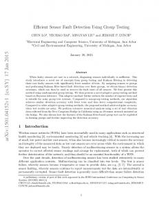
To evaluate residuals and to obtain information about faults, simple thresholding can be applied. If residuals are smaller than the threshold value, a process is considered to be healthy, otherwise it is faulty. For fault detection, the residual must meet the ideal condition being zero in the fault-free case and different from zero in the case of a fault. In practice, due to modelling uncertainty and measurment noise, it is necessary to assign thresholds larger than zero in order to avoid false alarms ( Patan (2008), Basseville and Nikiforov (1993)). This operation causes a reduction in fault detection sensitivity. Therefore, the choice of the threshold is only a compromise between fault decision sensitivity and false alarm rate. In order to select the threshold, in this paper method of ς-standard deviation is used. Assuming that the residual is an N (m, v) random variable, thresholds are assigned to the values: T = m ± ςv (7) where m is mean value and v is standard deviation of residuals values and ς, in the most cases, is equal to 1, 2 or 3. The probability that a sample exceeds the threeshold is equal to 0.15866 for ς = 1, 0.02275 for ς = 2 and 0.00135 for ς = 3, respectively.

4.1 Selecting the threshold

1500

Fig. 3. Simulation residuals used for selecting of threshold. Table 3. Thresholds for diffrent ς values. ς 1 2 3

threshold range -0.0077 ÷ 0.0109 -0.0170 ÷ 0.0202 -0.0263 ÷ 0.0295

5. EXPERIMENTS The experiments were divided into two parts. The first group of experiments was aimed on creating the optimal structure of the neural network model. For the training purposes the training set based on the data generated from the simulator of the boiler unit implemented in Simulink was created. The training set was generated using the control signal in the form of random steps with the values from the interval [0;0.5] and consists of 1500 samples. The training was carried out off-line for 100 epochs with the Levenberg-Marquardt algorithm. To verify the networks performance Mean Square Error (MSE) function was used. In the experiments the best performance (the lowest value of MSE) was achieved for the network with 5 neurons in the hidden layer with hyperbolic tangent activation function. Designed model has 3 output states (third order model). The neural network model structure is presented in Fig. 4. The modelling efficency for the training data is shown in Fig. 5. 5.1 Fault detection

Based on residuals (set consisted of the 1500 samples) collected from the boiler simulator (Fig. 3), mean value m and standard deviation v are calculated as follows: N 1 X ri = 0.0016 (8) m= N i=1 N

1 X v= (ri − m)2 = 0.0093 N − 1 i=1

1000 time (samples)

4. FAULT DETECTION

(9)

In Table 3 thresholds values generated according to (7) with different ς levels are presented. Exceding threshold calculated with the value of ς equal to 1, one can achive the fastest fault detection, but with high probability of false alarm and for ς equal to 3, probability of false alarm is very low but detection time is relatively long.

Well trained neural model can be successfully applied to fault detection. During experiments faults were simulated at 600th time instant and lasted 400 time instants. The desired water level in the boiler unit is set to the value 0.25. As it has been described in Section 2, four faulty scenarios were investigated. In Figs 6 and 7 one can see the behaviour of the fault detection system in the case of faults f1 and f4 , respectively. There can be easily noticed that plant behaviour radically changes in the case of abnormal behaviour and one can see a large difference between plant and model outputs. For purpose of fault detection residuals are calculated according to (4). The next step is calculating performance indexes for different values of thresholds. In this work the following quality measures are used:

Output (dashed) and simulated output (solid) 0.3

0.25 e(k−1) 0.2 x3hat(k+1) 0.15

level (L)

u(k)

x3hat(k)

0.1

x2hat(k+1)

0.05

x2hat(k) x1hat(k+1)

0

x1hat(k) −0.05

0

500

1000

1500

time (samples)

Fig. 4. Optimal structure of the state space neural network model

Fig. 6. Fault scenario f1 : system output (solid line) and model output (dashed line). Output (dashed) and simulated output (solid) 0.4

0.3

0.35

0.25

0.3

0.2

0.25 level (L)

level (L)

Output (dashed) and simulated output (solid) 0.35

0.15

0.2

0.1

0.15

0.05

0.1

0

0.05

−0.05

0

500

1000

1500

time (samples)

Fig. 5. Simulation of model with training data. • detection time tdt - period of time needed for the detection of a fault measured from tf rom which is the time of the fault start-up, to a permanent, true decision about a fault. • false detection rate rf d defined as follows: P i i tf d (10) rf d = tf rom − ton where tif d is the period of the i-th false fault detection and ton is the simulation start-up. Its value shows the percentage of false alarms. • true detection rate rtd P i i ttd (11) rf d = thor − tf rom where titd is the period of the i-th true fault detection and thor is time horizon after which simulation is out of interest. This index is used in the case of faults and describes the efficency of fault detection. Performance indexes are shown in Table 4. Examples of fault detection using different thresholds are shown in Fig. 8 and Fig. 9.

0

0

500

1000

1500

time (samples)

Fig. 7. Fault scenario f4 : system output (solid line) and model output (dashed line). Table 4. Performance indexes for fault examples. fault f1

f2

f3

f4

ς 1 2 3 1 2 3 1 2 3 1 2 3

tdt 13 21 29 27 42 57 6 6 6 18 30 42

rf d 0.0768 0 0 0.0768 0 0 0.0768 0 0 0.0768 0 0

rtd 0.9700 0.9500 0.9300 0.9350 0.8975 0.8600 0.9875 0.9875 0.7900 0.9575 0.9275 0.8975

6. CONCLUSION As was shown through the experiments, the neural network based state space innovations form model of a dynamic system can be effectively and easily used to fault detection of the boiler unit. In the faulty situation investigated,

0.3

0.25

residuals

0.2

0.15

0.1

0.05

0

−0.05

0

500

1000

1500

time (samples)

Fig. 8. Residual and thresholds for ς=1 (dotted line), ς=2 (dashed line) and ς=3 (solid line).

0.04 0.02 0

residuals

−0.02 −0.04 −0.06 −0.08 −0.1 −0.12 −0.14

0

500

1000

1500

time (samples)

Fig. 9. Residual and thresholds for ς=1 (dotted line), ς=2 (dashed line) and ς=3 (solid line). model behaved pretty well and using a simple thresholding technique it was possible to discover the fault. Our future research interest will focus on the investigation of proposed modelling approach to fault detection of incipient fault as well as application of state space neural networks models to fault tolerant control system design. REFERENCES Basseville, M. and Nikiforov, I.V. (1993). Detection of Abrupt Changes: Theory and Application. Prentice Hall, Englewood Cliffs. Blanke, M., Kinnaert, M., Lunze, J., and Staroswiecki, M. (2006). Diagnosis and Fault-Tolerant Control. Springer, Berlin. Bouthiba, T. (2004). Fault location in ehv transmission lines using artificial neural networks. International Journal of Applied Mathematics and Computer Science, vol. 14, pp. 69–78.

˙ Koj, J., Zelazny, M., and Ko´scielny, J. (2005). Laboratory stands for research and didactic purposes in the area of automatic control and diagnosis. Measurements, Automatic Control, Monitoring, 50(9), 261–264. Special issue, in Polish. Korbicz, J., Koscielny, J.M., Kowalczuk, Z., and (eds) Cholewa, W. (2004). Fault Diagnosis. Models, Artificial Intelligence, Applications. Springer-Verlag, Berlin. Leszczy´ nski, M. and Syfert, M. (2005). Application of fault tolerant control system for the boiler laboratory setup. In Proc. XV National Control Conference, KKA’05, Warsaw, Poland, volume II, 175–178. In Polish. Ljung, L. (1999). System Identification - Theory for the User. Prentice Hall, Englewood Cliffs. Norgaard, M., Ravn, O., Poulsen, N.K., and Hansen, L.K. (2000). Neural Networks for Modelling and Control of Dynamic Systems. Springer-Verlag, London. Patan, K. (2007). Stability analysis and the stabilization of a class of discrete-time dynamic neural networks. IEEE Trans. Neural Networks, 18, 660–673. Patan, K. (2008). Artificial Neural Networks for the Modelling and Fault Diagnosis of Technical Processes. Springer-Verlag, Berlin. Patan, K., Witczak, M., and Korbicz, J. (2008). Towards robustness in neural network based fault diagnosis. International Journal of Applied Mathematics and Computer Science, 18(4), 443–454. Patton, R.J. (1997). Fault-tolerant control: the 1997 situation (survey). In Proc. IFAC Symp. on Fault Detection, Supervision and Safety for Technical Processes, SAFEPROCESS’97, Hull, U.K., 1029–1052. Polycarpou, M. and Vemuri, A.T. (1995). Learning methodology for failure detection and accommodation. IEEE Control Systems Magazine, 15, 16–24. Theillol, D., C´edric, J., and Zhang, Y. (2008). Actuator fault tolerant control design based on reconfigurable reference input. International Journal of Applied Mathematics and Computer Science, 18(4), 553–560. Witczak, M. (2006). Advances in model-based fault diagnosis with evolutionary algorithms and neural networks. International Journal of Applied Mathematics and Computer Science, vol. 16, pp. 85–99. Zamarreno, J.M. and Vega, P. (1998). Fault location in ehv transmission lines using artificial neural networks. Neural Networks, vol. 11, pp. 1099–1112. Zhang, Y. (2007). Active fault-tolerant control systems: integration of fault diagnosis and reconfigurable control. In J. Korbicz, K. Patan, and M. Kowal (eds.), Fault Diagnosis and Fault Tolerant Control, ISBN: 978-8360434-32-1, Challenging Problems of Science - Theory and Applications : Automatic Control and Robotics, 21– 41. Academic Publishing House EXIT, Warsaw.