ologies have been developed to test signal integrity in high-speed SoCs. Testing ..... In [15] and [1], the worst case test patterns associated with a specific.
Signal Integrity: Fault Modeling and Testing in High-Speed SoCs Mehrdad Nourani and Amir Attarha Center for Integrated Circuits & Systems The University of Texas at Dallas Richardson, TX 75083-0688 nourani,attarha @utdallas.edu �
Abstract
[9] and shielding wires (e.g. grounding every other line) [12].
As we approach 100nm technology the interconnect issues are becoming one of the main concerns in the testing of gigahertz system-onchips. Voltage distortion (noise) and delay violations (skew) contribute to the signal integrity loss and ultimately functional error, performance degradation and reliability problems. In this paper, we first define a model for integrity faults on the high-speed interconnects. Then, we present a BIST-based test methodology that includes two special cells to detect and measure noise and skew occurring on the interconnects of the gigahertz system-on-chips. Using an inexpensive test architecture the integrity information accumulated by these special cells can be scanned out for final test and reliability analysis.
Noise and skew imposed by interconnects have emerged as main concerns in the interconnect design of gigahertz SoCs. Buffer insertion and transistor resizing methods [13] [14] are used as design techniques to achieve better power-delay and area-delay tradeoffs. Self-test methodologies have been developed to test signal integrity in high-speed SoCs. Testing crosstalk in chip interconnects [1][15] and a BIST (built-in self-test) structure using D flip-flops that detects the propagation delay deviation of operational amplifiers [16] are among such methods.
1.2 Contribution and Paper Organization Our main contribution is an on-chip mechanism to detect noise and skew violations occurring on the interconnects of high-speed SoCs. We present special cells to monitor signals received from the system interconnect and record the occurrence of signal entering the vulnerable region over a period of operation. By resizing transistors within these cells, they can be easily tuned to define the acceptable levels of noise and skew. We also propose a BIST methodology that uses pseudo-random patterns and accumulates the integrity test information using the detector cells. The statistics will be eventually sent out for final test analysis, reliability judgment and diagnosis.
1. INTRODUCTION With fine miniaturization of VLSI circuits and rapid increase in the working frequency (gigahertz range) of digital system-on-chips (SoC), the signal integrity becomes a major concern for design and test engineers. Although various parasitic factors for transistors can be well controlled during fabrication, the parasitic capacitances, inductances and their cross coupling effects on the interconnects play a significant role in the proper functionality and performance of high-speed SoCs. Signal integrity is the ability of a signal to generate correct responses in a circuit. It generally includes all effects that cause a design to malfunction due to the distortion of the signal waveform. According to this informal definition, a signal with good integrity has: (i) voltage values at required levels and (ii) level transitions at required times. For example, an input signal to a flip-flop with good signal integrity arrives early enough to guarantee the setup and hold time requirements and it does not have spikes causing undesired logic transition.
The rest of this paper is organized as follows. The signal integrity model and test strategy are discussed in Section 2. In Section 3 we explain the issue of generating patterns that stimulate the maximal integrity loss on interconnects. Section 4 and 5 analyze CMOS circuits that detect noise and skew violations occurring on the interconnects, respectively. Section 6 explains the test architecture to store and read out the information. The experimental results are discussed in Section 7. Finally, the concluding remarks are in Section 8.
1.1 Prior Work Various signal integrity problems have been studied previously for radio frequency (RF) circuits and recently for high-speed deep-submicron VLSI chips. The most important ones are: crosstalk (signal distortion due to cross coupling effects between signals) [1] [2], overshoot (signal rising momentarily above the power supply voltage) [3] [4], reflection (echoing back a portion of a signal), electro-magnetic interference (resulting from the antenna properties) [5], power supply noise [6] and signal skew (delay in arrival time to different receivers) [7][8].
2. INTEGRITY TEST METHODOLOGY 2.1 Interconnect Model Signal integrity problems originate from the circuit interconnects [17]. A wire not only serves as a conductor of electrons but also includes parasitic resistor (at low frequencies), capacitor (at mid-range frequencies), inductor (at high frequencies) and antenna (at very high frequencies), all of which can affect signal integrity. In low and mid-range frequencies, common in the past, the RC delays have been the dominating factors in the global interconnect delay and distortion. Inductance (L) effects are becoming increasingly important as frequency of operation increases.
There is a long list of possible design and fabrication solutions to enhance signal integrity on the interconnect. None guarantees to resolve the issue perfectly. These solutions include: 3-D layout modeling and parasitic extraction [9], accurate RLC simulation of on-chip power grid [7], using decoupling capacitors to limit the maximum dV dt [10][6] and to improve IR-drop [7][11], inserting buffers on the interconnects
There are many efficient distributed models in the literature [18][19] [20]. Figure 1 shows an accurate equivalent RLC circuit for several parallel interconnect lines [18][21]. This model comprises resistance (R), partial self inductance (L) and capacitance (C) for each segment, mutual inductances (M) and coupling capacitance (Cc ) between all
�
1
.. . Line i-1
.. . R
L
R
.. .
C
Line i
R
Cc2 M1
L
R
Line i+1
R
Cc2 M1 R
L
R
L
An RLC segment
Vdd VHmin
Cc2
Cc1 M2
L
... C
Cc1
M1
C
.. .
Cc1 M2
C Cc1
M1
... C
L
C
VHthr
L
C Cc1 M2
M1
R
L
R
VLmax
Cc1
M1 L
C
.. .
...
Vss VLthr
C
.. .
overshoot
ringing excessive delay
� �� � �� � �� �� � �� � �� � �� �� � �� � �� ��� � � �� �� �� �� �� ��� �� �� � � � �� � ��� ��� � � � � � �� � �� � �� �� � �� � �� ��� � � � �� ��� ��� � � � �� � �� �� � �� � ��� ��� � � � � � �� � �� �����
�� � � � � � ���� �� �
T_SI_R
T_SI_F
- Noise-Immune (NI) Region: - Skew-Immune (SI) Region:
Figure 1: An interconnect model.
- Ideal signal: - Signal with acceptable integrity: - Signal with unacceptable integrity loss: (occurrence of integrity fault)
pairs of parallel components. The values of distributed R, L and C depend on many factors including the operating frequency, length and technology. The number of segments can be selected based on the length of the interconnect and the operating frequency. All results reported in this work are based on this distributed RLC model [18][21].
- VHmin/VLmax: Minimum/Maximum input voltage guaranteed to be recognized as 1/0 - VHthr/VLthr: Acceptable positive/negative overshoot - T_SI_R/T_SI_F: Skew immune range (rising/falling)
2.2 A Model for Signal Integrity
Figure 2: Immune regions and the concept of integrity loss.
True characteristics of a signal is reflected in its waveform. Recent interconnect simulation, design and optimization methods not only consider peak voltage and delay, but also take into account the signal waveform [22] [23]. In reality, electronic components can tolerate certain level of noise. For example, a CMOS gate interprets any voltage in the VHmin Vdd range as logic “1” and any voltage in the Vss VLmax range as logic “0”. Frequently, digital circuits are designed to tolerate certain amount of skew delay, i.e. TSI R for rising delay and TSI F for falling delay (see Figure 2).
�
0 10
∆f/f (normalized)
� �
� �� � �� �� � �� � �� �� � �� ��� �� �� �� ��� �� �� �� �� � ��� ��� � � � �� � �� �� � �� ��� �� �� ��� ��� � �� �� �� � ��� ��� � � � �� �����
�
-1 10
-2 10
In practice, circuits have noise-immune (NI) regions that tolerate certain level of voltage swing and skew-immune (SI) regions that tolerate certain level of delay. Any portion of signal that exits the NI and SI regions indicates the integrity loss. This concept has been shown graphically in Figure 2 in which the shaded and unshaded (white) strips show the immune and vulnerable regions, respectively.
NOT: NAND: NOR:
0 10
1 10
2 10
Time (year)
Figure 3: The effect of overshoots on performance and life time.
The focal point in this paper is the NI and SI regions, covering integrity faults on interconnects, and a mechanism to detect signals that exit these regions. Leaving the NI-region not only causes error in functionality (ringing), but also shortens system’s life time due to timedependent dielectric breakdown (TDDB) [24]. More importantly, repeated overshoots are known to inject high-energy electrons and holes (also called hot-carriers) into the gate oxide that ultimately cause permanent degradation of MOS transistors’ performance and reliability [3]. For example, in [3], the authors presented the life time analysis, illustrated in Figure 3, showing that the performance of logic gates under stress (e.g. repeated overshoots) degrades quickly which eventually causes failure in the system.
system performance. However, the ATE (automatic test equipment) speeds have always lagged behind the CUT (circuit under test) speed. As a result of this speed difference, the high-speed circuits are tested at clock rates that are much slower than their specification [25] [26]. Furthermore, the pin and probing limitations of ATEs restrict the accurate observation of test results. Therefore, an on-chip test mechanism such as BIST can fulfill requirements for at-speed testing of complex high-speed SoCs. In a BIST architecture, a TPG (test pattern generation) circuit generates the pseudorandom patterns to stimulate possible defects in the CUT. The ORA (output response analyzer) circuit observes the outputs and analyzes their validity [27]. Figure 4 demonstrates our basic BIST-based architecture to test the SoC’s interconnects for integrity. The TPG and ORA circuits are located in two sides of the IUT (interconnect under test). The IUTs could be long interconnects or those suspicious of having noise/skew violations due to environmental factors (e.g. crosstalk, electromagnetic effects, etc.).
Leaving the SI-region means that the interconnect adds unacceptable skew delay that may lead to functional error or serious performance degradation. The range of immunity (TSI ) depends on the system topology, speed, core interactions and the yield margin that designer defines in the design phase. However, delay values of components as well as interconnects may not eventually be kept within such bound since the layout generation tools and the fabrication process each may add additional delays.
Our rationale in using pseudorandom patterns for integrity testing is the fact that finding patterns that are guaranteed to create the worst case scenarios for integrity loss (e.g. noise and skew) is impractical with the current state of knowledge. This is mainly due to the complexity of distributed RLC interconnect model, parasitic values and too many influential factors. We elaborate on this in Section 3.
2.3 BIST-Based Test Methodology At-speed testing (testing system functionality at its nominal working frequency) is a necessity for manufacturing test and validation of 2
T P G
(Interconnect Under Test) IUT
1
ND cell FFs SD cell
O R A
h 11 (s)
2
h 1m (s)
1 2
H(s)= h n1(s)
h nm (s)
m
n
BIST controller
Figure 5: Transfer function of an interconnect network
Figure 4: Proposed BIST architecture.
ods), the transfer function of a specific output f r (1 � r of order q:
Integrity loss cannot be captured using conventional ORAs due to the complexity of interconnect behavior. Hence, a new ORA circuitry, which includes ND (noise detector) and SD (skew detector) cells will be used in this work. The ND and SD cells detect voltage and timing violations of the signal, respectively. We will elaborate on their structures and behaviors in Sections 4 and 5.
h fr s ���
3. TEST PATTERN GENERATION
q
ki j pi j �
(1)
where ki j and pi j are residues and poles of the output f r , respectively. Note that h fr s � is obtained based on the superposition of the effects of all n inputs on fr . The output of system can be computed in the frequency domain by multiplying the transfer function and an input function. After transferring it to time domain to observe the timing behavior of the output, f r t � is calculated:
Researchers have searched for test patterns causing the worst case of signal integrity loss to enhance their test quality. In this section, we first present an analytical (but expensive) methodology to find deterministic patterns for maximal integrity loss. We then examine the inaccuracy of the RC model to conclude that the conventional TPG could be behaviorally effective and cost efficient.
fr t ���
3.1 Deterministic Pattern Generation
n
∑ �
i 1
Coping with sophisticated RLC network leads to impractical simulation time for long interconnects. For an analytical approach, we propose to utilize the model order reduction strategy as an alternative for circuit simulators to improve the simulation run time significantly. Model order reduction methods were developed to approximate the behavior of long interconnect, power and clock networks. They have been extensively used in the simulation and evaluation of high-speed VLSI systems [32][33][35]. They comprise the key factors of the original system with much lower complexity; therefore, they significantly reduce the required computation and thereby simulation time, with slight loss of accuracy. Elmore delay model [36], as the first reduced order model, is the most common technique for approximating the delay of RC networks. Asymptotic Waveform Evaluation (AWE) [32] was introduced as another method based on moment-matching allowing a linear circuit to be analyzed for its dominant poles and corresponding residues. To overcome some numerical limitations that AWE method suffers, researchers have developed reduction methods based on Bi-orthogonalization algorithms such as Pade Via Lanczos (PVL) [35] or orthogonalized Krylov subspace methods [37], which are computationally convenient and numerically better behaved. Their experimental results reveal the high accuracy within less than 5% of SPICE simulator at the speed 1000 times faster. For analytical computation, the reduced order model can be used in generating test patterns for maximal integrity loss on long interconnects deterministically. The details are beyond the scope of this paper and can be found in [38]. Briefly, the input to an interconnect network, i t � , can be expressed as: i t ��� ai u t ��� bi , where u t � is a step function, ai ��� 1 0 1 � and bi � � 0 1 � (if ai �� 1 then bi � 0).
� �
n
∑∑ i� 1 j � 1 s
� m) becomes
�
An interconnect network can be represented by a set of transfer functions in the S-domain. As shown in Figure 5, the interconnect network with n inputs and m outputs is represented by H S � , which contains n � m transfer functions relating n inputs and m outputs. Note that in general we have m � n for the possibility of fanout on some wires. Using an order reduction method (e.g. PVL [35] or ENOR [33] meth-
�
q
ai
∑ �
j 1
ki j exp pi j t � pi j �
q
1��� bi ∑ ki j exp pi j t ��� j� 1
f or t
� 0
(2)
By Equation 2, all the timing information of the output signal is available and the impact of inputs are considered within ai and bi coefficients. Therefore, theoretically we are able to analyze the output for any possible indication of signal integrity loss such as delay, overshoot, or undershoot. For example, maximal delay due to integrity loss can be obtained by equating the Equation 2 to 0 � 5Vdd and using numerical method to solve it for t. The reduced order model is much faster than SPICE simulation but this solution is still too expensive with the current state of knowledge of optimization, numerical methods and computers. For proof of concept, we have selected a small example of two parallel interconnects of five RLC segments each. We used the ENOR algorithm [33] to obtain the residues and poles of the 5th order reduced form of Equation 2. Two experimentations were done. First, we used SPICE [39] to exhaustively check all patterns for maximal delay. Second, ENOR was implemented using MATLAB [40]. After obtaining the poles and residues of the reduced order model, the information is used to solve the Equation 2 to calculate the delay and overshoot in the MATLAB environment. The maximum delay and peak overshoot (O.S.) are reported in Table 1 for three arbitrary transitions. As this table shows, our method identifies the same test patterns to stimulate the maximal integrity loss as SPICE finds but runs much faster. The running time for each run for SPICE and our order reduction method are 410 and 3 seconds (wall clock time on SPARC ULTRA 10 with 64 MByte RAM), respectively. While our analytical method is very accurate and is efficient for small examples, we acknowledge that finding patterns for large set of interconnects is very computational intensive using this approach unless more efficient numerical methods to solve Equation 2 is found. This is the main reason that we used pseudorandom patterns, generated by conventional TPG, in our approach.
3.2 Inaccuracy of Single-Victim (RC) Model In [15] and [1], the worst case test patterns associated with a specific fault model (MAFM) were presented. They used the RC interconnect for test pattern generation. Techniques, such as the one reported 3
2
Table 1: Comparing SPICE and our reduced method. Test SPICE Order Reduction Patterns Delay [ps] O.S. [Volt] Delay [ps] O.S. [Volt] 00 01 32.43 2.53 31.97 2.59 00 11 39.98 2.65 38.62 2.64 01 10 44.65 2.89 45.06 2.91 Test for Positive Noise (Glitch) Crossing VLmax W1
1.5
Volts
1
0
Test for Excessive Skew (Delay)
Crossing VHmin Crossing TRmax
0.5
Crossing TFmax
-0.5
...
...
...
...
...
... -1
Wi-1
1
0
1
0
Wi (Victim) Wi+1
Test for Negative Noise (Glitch)
Crossing VHthr Crossing VLthr
Random:1100000-->0011111 RC:1111011-->0000100
...
...
...
...
...
...
0.4 0.6 Time [ns]
0 1
1 0
1 1
0 1
0 0
1 1
1 0
0 1
1 0
1 0
0.8
1
Figure 7: Comparing patterns for the worst case delay.
Wn Victim (Wi): 0 Others (Wj;j = i): 0
0.2
0
0 1
0.8
Random:1110001-->0001010 RC:0000000-->1111011
0.6
Figure 6: Creating maximal integrity loss using RC model.
0.4 Volts
in [15], apply identical transitions to all wires except the victim net to create maximal integrity loss in the victim wire. Six scenarios and typical test patterns used in such techniques (e.g. [15]) have been shown in Figure 6. Although this set of test patterns can test interconnects at lower frequencies where inductance is negligible, it is inadequate for higher frequencies. Our empirical evidences show that in high frequency they fail to show the true picture of integrity of a signal.
0.2 0 -0.2 -0.4 -0.6
For accurate analysis, having the coupling capacitances between all wires in a distributed model (e.g. Figure 1) is necessary but not sufficient. The effect of capacitive coupling is considered local, in the sense that the coupling effects of adjacent wires are quite dominant compared to the capacitive coupling effects of far off wires [18][41]. However, the inductance has larger range effect and thus the effect of mutual inductance could be significant. As discussed in [18], the effect of coupling inductances and capacitances on a wire oppose each other. When the signal on a wire switches in one direction, the noise due to capacitive coupling affects other nearby signals in the same direction as that of switching while the noise due to inductive coupling is in the opposite direction. All of these make the patterns generated by RC models inaccurate and inadequate.
0
0.2
0.4 0.6 Time [ns]
0.8
1
Figure 8: Comparing patterns for the maximal noise.
Figure 7, test pattern pair 1100000 delay than the RC patterns.
0011111 can generate 31% more
Example 2: Maximal Noise In Figure 8, the difference between the worst case test pattern for RC model and another test data is demonstrated. In this case, the glitch on quiescent line 3 at 0 is investigated. This example shows that the worst case patterns (in terms of peak and duration of noise) for RC model are not necessarily the worst case for RLC model. �
In what follows, we present three other experiments to show the deficiency of RC model and the corresponding uniform patterns. These examples clearly show that there are scenarios for test patterns that create worse delay and/or noise on the signal and cause more integrity loss compared to those commonly reported earlier [15][18]. Thus, RLC model of interconnect needs to be consolidated for test pattern generation. We have used an RLC model of seven parallel interconnect lines (indexed “7654321”) for our experimentation. The R, L and C values are extracted using accurate extraction tools [28]. TISPICE has been used to simulate the complete RLC model. Typical CMOS gates are considered as driver and driven gates in two sides of the interconnect and Vdd � 1 � 2 Volt. Note that in the waveforms of these examples RC refers to the test pattern (similar to those in Figure 6) suggested by approaches that use RC interconnect modeling. We call them RCpatterns for short. Note that many random patterns stimulate integrity loss (noise) more than limited RC-patterns. We will show some statistics in Section 7.
Example 3: Mutual Effects We believe categorizing lines as victim and aggressors is misleading and unrealistic. Every line (including so-called aggressors) can be affected by all other lines (including so-called victims). Although the overall effect of aggressors on victims may be larger than effect of victims on aggressors, the change on the other lines cannot be ignored. Such minor effects may cause different switching times for aggressors which eventually results in longer settling delay up to 51% as reported in [18]. Figure 9 shows an example in which line 5 is quiescent at 1 and lines 4, 6 and 7 make 1 0 transitions. As shown in the figure, they affect each other due to the inductive and capacitive couplings. �
In conclusion, due to the complexity of accurate RLC interconnect model, parasitic values and too many influential factors, finding patterns guaranteed to create the worst case scenarios for noise (integrity loss) is very much difficult and almost impractical with the current state of knowledge. Our empirical evidences indicate that random patterns are more qualified than those conjectured (e.g. RC patterns in
Example 1: Maximal Delay Test pattern pair 1111011 0000100 is proposed for observing the highest potential delay on line 3 based on RC model. As shown in �
4
4
1.6
Line 4 Line 5 Line 6 Line 7
1.2 1 0.8 Volts
Input (Vb) Output (Vc)
3.5 3
Noise Detector (ND) Input/Output [volt]
1.4
0.6 0.4 0.2 0
VHthr
2.5
2 VHmin 1.5 1 0.5 0
-0.2
-0.5
-0.4 0
0.2
0.4
0.6
0.8
-1
1
0
2
4
6
8
Time [ns]
Figure 9: Mutual effects of wires. Signal a
b
c
Core j
18
20
W-set 1 ; Vdd=2.5 W-set 2 ; Vdd=2.5 W-set 3 ; Vdd=3.3 W-set 4 ; Vdd=3.3 3
T3
T4 2.5
y x
T1
T2
SE
Test_mode
16
3.5
Vdd
T6
T7
14
Signal + noise
IUT
Signal Sample
To read-out circuit
12
Figure 11: The SPICE simulation of the ND cell for the top vulnerable region.
� � �
Output (Vc) [volt]
Core i
10 Time [ns]
x
T5
2
1.5
Gnd 1
Figure 10: The ND cell using cross-coupled PMOS amplifier. 0.5 1
1.5
2
V- =VHmin=1.60
Figure 6) to create the worst case integrity loss. Thus, we propose to use conventional TPGs to generate pseudorandom test patterns as an efficient way to test the high-speed interconnects. We will elaborate on this issue in Section 7.
3
3.5
4
V+ =VHthr=2.75 Input (Vb) [volt]
Figure 12: The hysteresis property of our noise detector cell.
the hysteresis curve shown in Figure 12. This property helps to detect the violation of two threshold voltages (i.e. VHthr and VHmin ) with the same ND cell. For example, the solid-line curve shows that the switching threshold voltages are V � VHthr � 2 � 75 and V � VHmin � 1 � 60 when Vdd � 2 � 5. A similar cell can be designed to detect crossing VLthr and VLmax threshold voltages. Details can be found in [31].
4. DETECTING NOISE VIOLATION A modified cross-coupled PMOS differential sense amplifier is designed to detect integrity loss (noise) relative to voltage violations. Figure 10 shows the noise detector (ND) cell, which sits physically near the receiving core and samples the actual signal plus noise received by Core j. NMOS transistor T5 is the current source (when SE � 1) and PMOS transistors T3 and T4 are loads. The positive feedbacks (drain-gate connection between T3 and T4 ) allow amplification in this structure. SE is connected to test mode to create a permanent current source in the test mode and input x is connected to Vdd to define the threshold level for sensing Vb , i.e. the voltage received in x. The inverter, formed by T6 and T7 , stabilizes the voltage levels in the output of ND cell. By adjusting the size of the PMOS transistors (i.e. W and L), the current through transistors T1 and T2 are set to different values. Combining this with the feedbacks between PMOS transistors creates threshold voltages to turn the transistors on or off. Various architectures for sense amplifiers and in-depth details can be found in [29][30].
�
�
What level of overshoot is acceptable, and what level of voltage should be recognized as a logic “1” and “0” is debatable. Specific choice of VHthr and VLthr (and also VHmin and VLmax ) depends on the technology, and on the desired level of reliability. A nice feature of our ND cell is that for any Vdd , the two thresholds (i.e. V and V of hysteresis) can be tuned by changing the layout size of the PMOS transistors (mainly W’s of T3 and T4 ). This is also shown in Figure 12, in which different sets of transistor widths (W set 1 through W set 4 for T3 and T4 ) and two Vdd values (3.3 and 2.5 volts) have been used. There are analyticaland simulation-based approaches that can be used for such tuning [29]. Empirically, however, for a given Vdd we found tuning of V and V to be easy and flexible within a relatively large range as shown in Figure 12.
�
�
�
Figure 11 shows signals on the input and output (points b and c) of the cell to validate the behavior of our noise detector cell. Each time that noise occurs (i.e. Vb � V � VHthr ), the ND cell generates a “0” signal that remains unchanged until Vb drops below V � VHmin . The waveforms in Figure 11 reflect that the ND cell shows a hysteresis (Schmitttrigger) property which implicitly indicates a (temporary) storage behavior. To confirm this we ran a DC analysis on the ND cell to get
�
2.5
�
Note carefully that occurrence of an overshoot puts the ND cell in state-0 (i.e. generating “0”) after which a 1-0-1 glitch that violates VHmin can be detected. For detecting 1-0-1 glitches on a quiescent line, even without occurrence of overshoot, we need to tune the cell such that VHthr � Vdd . This forces the cell to go to state-0 for a quiescent logic-1 line and therefore make it capable of detecting 1-0-1 glitches.
�
5
40 35
T_interconnect
Core i
Gate Delay: Interconnect Delay: (Al & SiO2)
Core j T_comb
IUT
30 clock
Delay 25 [ps] 20
Storage Element: Clock-Output Delay: T_CQ Setup Time: T_Setup T_CQ T_interconnect
15
T_comb
T_setup T_SI
10 T_clock
5 0 650
500
350
250
180
130
The earliest time that data is ready in the output of Core i
100
The earliest time that data can be stored in Core j
Technology [nm]
Figure 14: The effect of interconnect skew (delay). Figure 13: Gate and interconnect delay versus technology. Signal Core i
Skewed signal
IUT
a
The drawback, however, is that the ND cell won’t be able to have VHthr larger than Vdd . If both features are desired we need two cells one to detect overshoots with user-defined VHthr and one for any 1-0-1 glitch that may occur.
Vdd
Vdd
T3
T1 d
Clock
5. DETECTING SKEW VIOLATION
T2
As stated in Section 1, in addition to voltage distortion, timing violation (skew) is another important factor that contributes directly to the integrity loss. Specifically, in deep sub-micron technology the interconnect delay is a detrimental factor. Figure 13, presented in the SIA roadmap [25], shows the gate and interconnect delays versus technology generations. The curves clearly show the dominance of interconnect delay over gate delay as we approach 100nm technology. Using copper (instead of aluminum) and low dielectric constant insulators can reduce the delay of interconnects. However, it is certain that the interconnect delay will remain the dominating factor [25]. This trend justifies the efforts needed to detect the delay violation due to the interconnect.
Core j
b
T4 T6
c
To read-out circuit
T5
��
�
Gnd Delay generator circuit (odd number of inverters)
Gnd (NOR gate)
Figure 15: Skew Detector circuitry (SD cell).
TSI �
�max� � Tclock
s to s
Tcomb max � TCQ � Tsetup �
�
5.2 Skew Detector (SD) Cell In designing high speed cores, very firm delay budget has to be met. Any minor violation of skew or unpredictable delay (e.g., the interconnect effect) may cause functional error or significant degradation of performance. Numerous research endeavors have been dedicated to the testing of logic gates for their timing behavior [43][44]. Since the interconnect skew delay will be the dominant factor in determining the clock period of future technologies, it is essential to detect the skew violation on the interconnects.
5.1 Skew Immunity Range We defined the skew-immune (SI) region in Figure 2 as the delay range that is considered “acceptable”. If signal skew goes beyond that range we consider it as serious integrity loss. The range of immunity depends on the system topology, speed, core interactions and the yield margin that a designer defines to achieve the nominal performance of the system. Such yield margin is often considered in the design phase. However, the delay values of components as well as interconnects may not eventually be kept within such bound since the layout generation tools and the fabrication process each may add additional delays. More importantly, as we have discussed in [31] signal integrity factor in general and noise/skew in particular are data-dependent phenomena that cannot be predicted accurately through analytical or simulation based approaches. Thus, similar to the noise detection only an on-chip methodology can successfully test the delay violation.
Detecting the skew violations of interconnects can unlikely be fulfilled off-chip due to the speed limitations of ATEs. Nevertheless, the features of an on-chip test mechanism such as BIST can be utilized to observe the skew violations accurately. Figure 15 depicts the proposed on-chip test circuitry (SD cell). A delay generator cell is used to create the desired delay value (i.e. acceptable skew-immune range TSI ) as it is defined by a designer based on the delay budget of the interconnect. This cell is essentially made of odd number of cascaded CMOS inverters that receives the system clock and outputs the delayed inverted clock. The delayed clock is compared with the interconnect output. If the skew of the signal on the interconnect output is not within the acceptable range, the SD cell issues a pulse. The duration of this pulse depends on the interconnect delay. From testing point of view, the pulse generated by the SD cell can be used as the indication of skew violation. For example, it can trigger a D flip-flop to store a “1” as indication of such occurrence.
In synchronous systems, maximum communication speed between two interacting cores depends on the maximum storage-to-storage (s-tos) path delay [42]. Figure 14 shows this graphically. As long as Tclock � Tinterconnect � Tcomb max � TCQ � Tsetup the functionality of system will remain error-free. For simplicity, we did not differentiate between rising and falling skews. Thus, the skew immune range TSI can be estimated based on the clock period, timing behavior of the storage elements and storage-to-storage paths within the system: 6
Table 2: Statistics for four delay generator circuits. Design # of Inverters Area [µm2 ] Delay [ps] #1 1 6 42 #2 1 2 87 #3 3 10.5 250 #4 3 15 410
CLOCK
VD
SIGNAL1
OUTPUT1
employed the classic driver design [46] [47] to implement the delay generator circuit. Many researchers have extensively investigated how to achieve the optimal driver for long VLSI interconnects considering different objectives such as minimum delay, area or power consumption [45] [47]. For instance, several design parameters, such as the number of drivers and their aspect ratio, are adjusted using optimization techniques to obtain an optimal driver configuration. Similarly, obtaining a specific delay value for a driver, while minimizing the overall area can be another objective in driver design problem. This can be the goal in optimizing the delay generator circuit. Such optimization technique, although important in our application, is beyond the scope of this paper. We simply comment that optimizing delay generator circuit can be done systematically using optimal driver design concept [13] [47].
SIGNAL2
OUTPUT2
54
108
162
216
270 324 PICO SECONDS
378
432
486
Figure 16: The SPICE simulation of SD cell for two signals.
4.0
3.5
NAME
LP/PS DB RR MD
CLOCK
0
1
0
SIGNAL1
0
1
0
OUTPUT1
0
1
0
SIGNAL2
0
2
0
OUTPUT2
0
2
0
3.0
As for experimentation, we designed few delay generator circuits to show typical values for TSI . Table 2 shows the specifications of four different delay generators. We used cascaded inverters with different size transistors to design and tune them. As seen in this table, the variety of delay values (i.e. TSI ) can be created using the inverters with reasonable area.
2.5 V O L T S
2.0
1.5
1.0
As Figure 17 shows, the SD cell detects the skew violations by creating a pulse in its output momentarily. One efficient way to capture such violation is to use this pulse to trigger a flip-flop as shown in Figure 18(a). This circuit stores a “clock=1” in the flip-flop when delay violations (in range of TSI delay T 2) occur. Note that this is a sufficient range in our application. Here our concern is small but unacceptable delays due to integrity loss. Large delays can be always captured using functional or delay testing.
0.5
0.0 60
120
180
240
300 360 PICO SECONDS
420
480
540
�
Figure 17: The SPICE simulation of SD cell connected to an interconnect. The SPICE [39] simulation of the SD cell has been illustrated in Figure 16 for two signals. The first signal (SIGNAL1) does not violate the skew limit (TSI ) and thus the output of the cell remains zero. The second signal (SIGNAL2), however, exceeds the acceptable skew and the SD cell generates a pulse. As shown in the figure, this pulse appears in the output of the SD cell after delay associated with the NOR gate. Notice that possible clock skew does not have significant effect on the behavior of the SD cell. There are many approaches such as [13][45] to minimize the clock skew in a large chip. However, in the presence of clock skew TSI changes to TSI � Tclock skew where the Tclock skew is the skew on the clock wire attached to the SD cell. This change increases the acceptable skew range to which the cell reacts but the functionality of the cell remains intact.
The clock signal (instead of a permanent “1”) is intentionally connected to the input of D flip-flop to filter out pulses on c for some undesired scenarios. One such scenario, e.g. having a pulse when skew is in the immune (acceptable) range, is shown in Figure 18(d). Depending on the application, accuracy and test patterns one SD cell to detect skew violations on rising signals (Figure 18(a)) is often sufficient. However, if distinction between skew violations of rising and falling signals is needed, e.g. for diagnosis purposes, we need additional hardware. The reader can easily verify that the additional cell is the same as Figure 18(a) but uses b d instead of b � d and can detect skew violations on falling signals.
To illustrate the true behavior of the SD cell in test mode, while connected to an interconnect, we ran the SPICE simulation on the integrated interconnect and test circuitry. The results are shown in Figure 17. If the output of interconnect does meet the skew requirements (less than TSI � 100ps as happens for SIGNAL1), the output of the SD cell stays at zero. However, a marginally late signal (SIGNAL2) causes a pulse at the output of the SD cell.
Detecting signals that leave the noise-immune (NI) and skew-immune (SI) regions is a crucial step. This is performed by the ND and SD cells explained in the previous sections. These cells are not expensive – seven and six transistors per ND and SD cells, respectively. Overall two cells are needed per interconnect to detect noise (crossing VHthr and VHmin ) and skew violations. The test architecture to read out the information stored in these cells is a DFT decision which depends on the overall SoC test methodology, testing objective and cost consideration.
�
6. TEST ARCHITECTURE
5.3 Delay Generator Circuit As discussed before the accuracy of the SD cell depends on accurate implementation of delay generator block. This circuit generates a specific delay value (e.g. TSI ), predefined by the designer. The implementation of such accurate delay circuitry is a challenging issue. We have
Figure 19 demonstrates a scan flip-flop chain architecture, which is able to record the occurrence of noise/skew violation and transfer it to the output. In the test-mode, first the flag signal is transferred, through MUX, to the test controller. If noise or skew violation (low integrity 7
Delay Generator (with delay of TSI )
b
clock D Q
Table 3: Integrity test results for 8051 bus structure. Buses Bitwidth Length [mm] Noise [%] Skew [%] Data 8 20 43.38 31.32 Address 16 5 23.28 15.78 Control 10 10 28.50 25.53 Internal 1 10 10 34.40 21.20 Internal 2 8 10 32.62 18.47 Average 10.40 11.00 32.44 22.46
Q
c
d clock (a) Immune Region
Immune Region
clock
clock
d
d
b
b
c
c
Q
Q
(b) Immune Region
Immune Region
clock
clock
d
d
b
b
c
c
Q
Table 4: Test overhead for 8051 bus structure. Overhead Data Address Control Int. 1 Int. 2 Cost [NANDs] 158 254 194 194 158 Time [Cycle] 1600 3200 2000 2000 1600
(c)
Q
(d)
it runs in 1 GHz. Typical global interconnect lengths in large SoC systems are chosen as the wire lengths in our experiments. Then, we have applied random patterns to the interconnects assuming that they run under 1 GHz frequency. The statistics are summarized in Table 3. As shown in Table 3, the average occurrence of unacceptable noise and skew (low integrity signals) in a presumed 1 GHz 8051 system will be 32.44% and 22.46% that may create functional error or cause severe damages (e.g. reliability, lifetime) on chip over time.
(e)
Figure 18: Capturing skew violations by the SD cell.
n-bit bus
.. .
ND-FF
ND Cell Vb Vc
Si
SD Cell Vb Vc
Si SD-FF So
.. .
So
.. .
ND Cell Vb Vc
Si So
SD Cell Vb Vc
Si
.. .
flag
0
Table 4 summarizes the test overhead for the buses in 8051 reported by SYNOPSYS design compiler toolset [49] when 100 random patterns are applied. We assumed that all interconnect lines need to be tested for integrity. All costs are expressed in terms of 2-input NAND gates. The readout time overhead results are also included in this table.
to scan-out chain
1
So Sout
Table 5 compares the quantity and quality of random test patterns versus the RC patterns for a 7-wire parallel interconnect line. The overall number of patterns used in this experiment are 42 (6 patterns per wire as shown in Figure 6) and 100 for RC and random cases, respectively. The second and third columns show the number of patterns that show significant integrity loss (i.e. overshoot or delay at least 15% larger than their nominal values) from different perspectives. Although in general, the number of the RC patterns is smaller than the random patterns, the latter significantly improves the quality of interconnect testing by stimulating larger integrity loss (the worst case scenarios). For example, when we average the results of applying all patterns (first row), the random patterns cause larger integrity loss (in terms of peak noise and settle time) than the RC patterns. As for maximal delay on the interconnects, 43 (out of 100) and 14 (out of 42) patterns were counted for random and RC cases, respectively, causing significant delay. The average delay caused by these patterns are 122ps versus 102ps. Similar trend exists for patterns that stimulate maximal peak/duration of noise.
Test Controller
Figure 19: Test architecture. signal) occurs ( f lag � 1), the content of flip-flops (ND-FFs and SDFFs) are scanned out through Sout for further reliability and diagnosis analysis. Suppose an n-bit interconnect is under test for m cycles (i.e. m pseudorandom test patterns). The very pessimistic worst case scenario in terms of test time is a case in which all lines are subject to noise in all m test cycles. This situation requires overall m and m n cycles for response capture and readout, respectively. In practice, a much shorter time (e.g. k n, where k m) is sufficient since the presence of defects or environmental factors causing unacceptable level of noise/skew (integrity loss) is quite limited. In terms of test overhead, n ND cells, n SD cells and 2n scan flip-flops are needed. �
�
Two other alternatives for the test architectures using compressor/adder and dedicated counters are introduced in [31] and analyzed for their cost and test time. Briefly, these alternatives are more expensive but can supply data of integrity loss occurrences more accurately for applications such as interconnect diagnosis, re-wiring and pad re-distribution.
7.1 The Effect of Process Variation Variation of different factors in the fabrication process may cause considerable deviation from the nominal or expected behavior of the circuit. This may affect the integrity of signals traveling on the interconnect and also the functionality of the ND/SD cells. For example, due to the limited resolution of the photolitographic process, the transis-
7. SIMULATION RESULTS The number of cores in the SoC and the number of input ports of cores do not influence the low-integrity (noise/skew) detection process since the ND and SD cells independently function near core input ports. They do, however, influence the cost of test overhead (e.g. cells and FFs) and test time (e.g. scan-out time).
Table 5: Integrity Factor Mutual Effects Maximal Delay Maximal Noise
The experimental results here are reported using OEA [28] and SPICE [39] simulators. We analyzed five main buses (data, address, control and two internal) of the famous 8051 microprocessor [48]. In our implementation the 7 cores communicate through these buses and are potentially subject to noise in high frequency. For experimentation purpose, we used the interconnect architecture of 8051 assuming that 8
Random test patterns versus RC test patterns. Quantity Quality RC Random Metric RC Random 42 100 Settle[ps] 61 117 Peak[V] 0 � 15Vdd 0 � 28Vdd 14 43 Delay[ps] 102 122 14
51
Settle[ps] Peak[V]
211 0 � 26Vdd
328 0 � 34Vdd
Table 6: The Effect of process variations on the interconnect. Parameters Nominal [µ] E[%] Peak Overshoot volt 1.62 24.7 Peak Undershoot volt 0.95 6.7 Skew Delay ns 0.4 4.7
Table 7: The Effect of process variations on the ND cell. Parameters Nominal [µ] E[%] Width (WT 1 WT 7 ) µm 4,4,8,7,4,1.2,4 6.2 Length µm 0.5 11.0 κ (NMOS, PMOS) (0.161,9.366) 2.1 Vth (NMOS, PMOS) volt (0.6684, 0.9352) 15.1
tor dimensions (W , L), on die may be different from the ideal dimensions expected. Other process parameters include transconductance (κ), threshold voltage (Vth ), impurity concentration on densities, oxide thicknesses and diffusion depths [29]. In this section we only show our simulation results on the sensitivity of the interconnect and cells with respect to different process variation factors. In-depth analysis of process variation is beyond the scope of this paper.
Table 8: The Effect of process variations on the SD cell. Parameters Nominal [µ] E[%] Width (W1 W2 W6 ) µm 1.5,1,2,2,1,1 5.0 Length µm 0.5 17.5 κ (NMOS, PMOS) (0.161,9.366) 0.6 Vth (NMOS, PMOS) volt (0.6684, 0.9352) 2.6
�
�
� �
�
�
�
�
�
�
�
�
�
In analyzing the effects of process variation on the SD cell, the delay generator cell (Figure 15)) is the key element that affects the overall accuracy of the cell. Monte-Carlo simulations were also carried out for the SD cell. Table 8 demonstrates the sensitivity of the SD cell in general, and its delay generator cell in particular, due to the process variations. As tabulated, the SD cell can adequately tolerate variations on width, κ, and threshold voltage. The percentage of unacceptable skewed signals is less than 5% for above factors. However, the variations on the length of SD cell seem to be larger.
�
8. CONCLUSION The rising level of complexity and frequency of chips makes it increasingly difficult to achieve an adequate interconnect test using the ad-hoc techniques currently practiced in industry. Signal integrity is often degraded as signal travels through the interconnect. Such integrity loss may lead to functional error and reliability loss. We proposed a systematic BIST-based methodology to model and test signal integrity in deep-submicron high-speed interconnects. On the test generation side, while deterministic patterns can be determined analytically, conventional cost-efficient pseudorandom pattern generator can stimulate the maximal integrity loss reasonably well. Using inexpensive built-in noise and skew detection cells we offered an efficient architecture to capture and scan out the occurrences of noise and skew violations.
7.1.1 The Effect on the Interconnect To examine the effects of process variations on the long interconnects parameters such as thickness, width, interlayer dielectric thickness, and contact resistance in fabrication process are taken into account as variances on the distributed R, L, and C values of the interconnect model. Table 6 shows the adverse effects of process variation on long on-chip interconnects when R L C values are varied randomly using normal distribution. E obtained in the simulation expresses the percentage of violations (overshoot, undershoot or skew that are 20% larger than their nominal values) occurred on the interconnects. For example, 24.7% of the inputs cause significant overshoots, which reduces chip reliability. �
�
�
�
� � �
In all simulation results reported here, a normal distribution with σ � 0 � 06µ is used to generate variation on such factors. This means that the change of the nominal value will remain in µ 3σ µ � 3σ range [50]. The average value (µ) is the result of simulation without any variation of parameters. The value for variance (σ) is selected to keep the random parameter values between a lower and upper bound. In practice, such bounds depend on the statistical data extracted for each fabrication plant [51]. The CODAC [52] and TISPICE [39] tools are used in a Monte-Carlo simulation environment to model and simulate the repercussion of process variations on the interconnects or cells. In each iteration the interconnect or cells is simulated using a randomlychosen value for that specific process factor.
�
�
�
Acknowledgements This work was supported in part by the National Science Foundation CAREER Award #CCR-0130513. The authors also thank Nagaraj NS (Texas Instruments, Inc.) and Jerry Tallinger (OEA International, Inc.) for providing their simulator packages and helpful comments.
Many researchers showed the importance of detecting skew and voltage violations of long interconnects on chips [53] [54]. Our simulation results also confirm this fact. Due to its probabilistic and environmentdependent nature, the process variation cannot be considered or modeled in the design phase. Thus, after fabrication a significant percentage of overshoots, violation of noise margin or settling time may appear on long interconnects. These situations can be only tested using an on-chip approach such as ours.
REFERENCES [1] M. Cuviello, S. Dey, X. Bai and Y. Zhao, “Fault Modeling and Simulation for Crosstalk in System-on-Chip Interconnects,” in Proc. Intern. Conf. on Computer Aided Design (ICCAD’99), pp. 297-303, Nov. 1999. [2] W. Chen, S. Gupta and M. Breuer,, “Test Generation in VLSI Circuits for Crosstalk Noise,” in Proc. Intern. Test Conf. (ITC’98), pp. 641-650, 1998. [3] P. Fang, J. Tao, J. Chen and C. Hu, “Design in Hot Carrier Reliability For High Performance Logic Applications,” in Proc. IEEE Custom Integrated Circuits Conf., pp. 25.1.1-25.1.7, Oct. 1998. [4] Yusuf Leblebici, “Design Considerations for CMOS Digital Circuits with Improved Hot-Carrier Reliability,” IEEE Journal of Solid-State Circuits, vol. 31, no. 7, pp. 1014-1024, July 1996. [5] S. Kimothi and U. Nandwani, “Uncertainty Considerations in Compliance-Testing for Electromagnetic Interference,” in Proc. Annual Reliability and Maintainability Symposium, pp. 265-268, 1999. [6] S. Zhao and K. Roy, “Estimation of Switching Noise on Power Supply Lines in Deep Sub-Micron CMOS Circuits,” in Proc. Intern. Conf. on VLSI Design, pp. 168-173, Jan. 2000.
7.1.2 The Effect on the ND cell To show the sensitivity of the ND cell with respect to the process variation, we have simulated the ND cell with variations of the different parameters. Using CODAC and SPICE, we trace the effect of variation of width (W ), length (L), transconductance (κ), and threshold voltage (Vth ) on the behavior of ND cell. Table 7 demonstrates the results. The last column in this table (E) shows the percentage of unacceptable outputs compared to the output of ND cell under no process variations for different parameters. As reflected in the table, the ND cell can quite adequately tolerate the variations on κ and length of transistors. However, the adverse effects of deviations of the threshold voltage and transistor width are larger.
7.1.3 The Effect on the SD cell 9
[7] H. Chen and L. Wang, “Design for Signal Integrity: The New Paradigm for Deep-Submicron VLSI Design,” in Proc. Intern. Symposium on VLSI Technology, pp. 329-333, June 1997. [8] D. Cho, Y. Eo, M. Seung, N. Kim, J. Wee, O. Kown and H. Park, “Interconnect Capacitance, Crosstalk and Signal Delay for 0.35 µm CMOS Technology,” in Proc. Intern. Meeting on Electron Devices, pp. 619-622, 1996. [9] L. Green, “Simulation, Modeling and Understanding the Importance of Signal Integrity,” IEEE Circuit and Devices Magazine, pp. 7-10, Nov. 1999. [10] R. Downing, P. Gebler and G. Katopis, “Decoupling Capacitor Effects on Switching Noise,” IEEE Transactions on Components, Hybrids and Manufacturing Technology, vol. 16, no. 5, pp. 484489, Aug. 1993. [11] R. Saleh, D. Overhauser and S. Taylor, “Full-Chip Verification of UDSM Designs,” in Proc. Intern. Conf. on Computer Aided Design (ICCAD’98), pp. 453-460, Nov. 1998. [12] A. Kahng, S. Muddu and E. Sarto, “Interconnect Optimization Strategies for High-Performance VLSI Designs,” in Proc. Intern. Conf. on VLSI Design, pp. 464-469, Aug. 1999. [13] G. Tellez and M. Sarrafzadeh, “Minimal Buffer Insertion in Clock Trees with Skew and Slew Rate Constraints,” IEEE Trans. on CAD, vol. 16, no. 4, pp. 333-342, April 1997. [14] Y. Jiang, S. Sapatnekar, C. Bamji and J. Kim, “Interleaving Buffer Insertion and Transistor Resizing into a Single Optimization,” IEEE Trans. on VLSI Systems, vol. 6, no. 4, pp. 625-633, Dec. 1998. [15] X. Bai, S. Dey and J. Rajski, “Self-Test Methodology for AtSpeed Test of Crosstalk in Chip Interconnects,” in Proc. Design Automation Conf. (DAC’00), pp. 619-624, 2000. [16] I. Rayane, J. Velasco-Medina and M. Nicolaidis, “A Digital BIST for Operational Amplifiers Embedded in Mixed-Signal Circuits,” in Proc. VLSI Test Symp. (VTS’99), pp. 304-310, 1999. [17] P. Nordholz, D. Treytnar, J. Otterstedt, H. Grabinski, D. Niggemeyer and T. Williams, “Signal Integrity Problems in Deep Submicron Arising from Interconnects Between Cores,” in Proc. VLSI Test Symp. (VTS’98), pp. 28-33, 1998. [18] C. Cheng, J. Lillis, S. Lin and N. Chang, Interconnect Analysis and Synthesis, John Wiley & Sons, 2000. [19] H. Veendrick, Deep-Submicron CMOS ICs: from Basics to Asics, Kluwer, 1998. [20] B. Sheehan, “Projective Convolution: RLC Model-Order Reduction Using the Impulse Response,” in Proc. Design Automation Conf. (DAC’99), pp. 669-673, 1999. [21] K. Gala, V. Zolotov, R. Panda, B. Young and D. Blaauw, “OnChip Inductance Modeling and Analysis,” in Proc. Design Automation Conf. (DAC’00), pp. 63-68, 2000. [22] J. Cong and L. He, “Theory and Algorithm of Local-RefinementBased Optimization with Application to Device and Interconnect Sizing,” IEEE Transactions on Computer-Aided Design of Integrated Circuits and Systems, vol. 18 no. 4, pp. 406-420, April 1999 [23] P.Restle, A.Tuehli and S. Walker, “Dealing with Inductance in High-Speed Chip Design,” in Proc. Design Automation Conf. (DAC’99), pp. 904-909, 1999. [24] W. Hunter, “The Statistical Dependence of Oxide Failure Rates on Vdd and Tox Variations with Applications to Process Design, Circuit Design and End Use,” in Proc. Reliability Physics Symposium, pp. 72-81, [25] Semiconductor Industry Association, The International Technology Roadmap for Semiconductors, Sematech, Inc., 1999. [26] A. Flint, “Testing Multichip Modules,” IEEE Spectrum, pp. 5962, March 1994. [27] M. Abramovici, M. Breuer and A. Friedman, Digital Systems Testing and Testable design, IEEE Press 1990. [28] OEA Interconnect Simulators, User’s and reference manual, OEA International, Inc., 2001. [29] J. Rabaey, Digital Integrated Circuits, Prentice Hall, 1996.
[30] P. Gray and R. Meyer, Analysis and Design of Analog Integrated Circuits, John Wiley & Sons, 2000. [31] M. Nourani and A. Attarha, “Built-In Self-Test for Signal Integrity,” in Proc. Design Automation Conf. (DAC’01), pp. 792797, June 2001. [32] L. Pillage, and R. Rohrer, “Asymptotic Waveform Evaluation for Timing Analysis,” IEEE Trans. on CAD, vol. 9, no 4, pp. 352366, April 1990. [33] B. Sheehan, “ENOR: Model Order Reduction of RLC Circuits Using Nodal Equations for Efficient Factorization,” Design Automation Conference, pp. 17-21, 1999. [34] P. Feldmann, and R. Freund, “Small-signal Circuit Analysis and Sensitivity Computations with the PVL Algorithm,” IEEE Trans. on Circuits and systems, vol. 43, no. 8, pp. 577-585, Aug. 1996. [35] P. Feldmann, and R. Freund, “Efficient Linear Circuit Analysis by Pade Approximation via the Lanczos Process,” IEEE Trans. on CAD, vol. 14, no. 5, pp. 639-649, May 1995. [36] W. Elmore, “The Transient Response of Damped Linear Networks With Particular Regard to Wideband Amplifiers,” Journal of Appl. Phys., vol. 19, no. 1, pp. 155-163, 1948. [37] A. Odabasioglu, M. Celik, and L. Pileggi, “PRIMA: Passive Reduced-Order Interconnect Macromodeling Algorithm, ” IEEE Conf. on CAD , 1997. [38] A. Attarha and M. Nourani, “Test Pattern Generation for Signal Integrity Testing,” Technical Report UTD-EE-2001-8-22, Department of Electrical Engineering, the University of Texas at Dallas, August 2001. [39] TI-SPICE3 User’s and reference manual, 2000 Texas Instrument Incorporation, 2000. [40] MATLAB User’s and reference manual, 2000 The MathWorks, Inc., Version 6.0.0.88,2000. [41] L. He, N. Chang, S. Lin and O. Nakagawa, “An Efficient Inductance Modeling for On-chip Interconnects,” in Proc. IEEE Custom Integrated Circuits Conf., pp. 457-460, 1999 [42] J. Wakerly, Digital Design, Principles and Practices, Prentice Hall, 2000. [43] U. Sparmann, H. Muller and S. Reddy, “Universal Delay Test Sets for Logic Networks,” IEEE Trans. on VLSI Systems, vol. 7, no. 2, pp. 156-166, Nov. 1999. [44] A. Majhi, and V. Agrawal, “Tutorial: Delay Fault Models and Coverage,” in Proc. 11th Internations Conf. on VLSI Design, pp. 364-369, 1998. [45] J. Lillis, C. Cheng and T. Lin, “Optimal Wire Sizing and Buffer Insertion for Low Power and a Generalized Delay Model,” IEEE Journal of Sold-State Circuits, vol. 31, no. 3, pp. 437 -447, March 1996. [46] V. Adler and E. Friedman, “Repeater Design to Reduce Delay and Power in Resistive Interconnect,” IEEE Trans. on Circuit and Systems-II: Analog and Digital Signal Processing, vol. 45, no. 5, pp. 607-616, May 1998. [47] D. Zhou, and X. Liu, “On the Optimal Drivers of High-Speed Low Power ICs,” in Proc. ICCAD’91 Conf., pp. 212-218, 1991. [48] Intel Corporation, “MCS-51 8-bit Microcontroller,”, Databook of Intel MCS-51 Microcontroller, 1994. [49] Synopsys Design Analyzer, “User Manuals for SYNOPSYS Toolset Version 2000.05-1,” Synopsys, Inc., 2000. [50] J. Devorce, Probability and Statistics for Engineering and the Sciences, John Wiley & Sons, 1999. [51] MOSIS Organization, USC Information Sciences Institute. Webpage URL address: http://www.mosis.org. [52] Texas Instrument Inc., CODAC User’s and Reference Manual, Texas Instrument Incorporation, 2000. [53] S. Natarajan, M. A. Breuer, and S. K. Gupta, “Process Variations and their Impact on Circuit Operation,” in Proc. IEEE Intern. Symp. on Defect and Fault Tolerance in VLSI Systems, pp. 73-81, 1998. [54] Nagaraj NS, P. Balsara, C. Cantrell, “Crosstalk Noise Verification in Digital Designs with Interconnect Process Variations,” in Proc. 14th Intern. Conf. on VLSI Design, pp. 365-370, 2001. 10
Biographical Sketch of Authors Mehrdad Nourani received his B. Sc. & M. Sc. degree in Electrical Engineering from the University of Tehran, Tehran, Iran in 1986. He received his Ph.D. in Computer Engineering from Case Western Reserve University, Cleveland, Ohio in 1993. During the academic year 1994, he was a postdoctoral fellow at Case Western Reserve University, Department of Computer Engineering. Dr. Nourani served Department of Electrical and Computer Engineering at the University of Tehran, Tehran, Iran from 1995 to 1998 and Department of Electrical Engineering and Computer Science at Case Western Reserve University from 1998 to 1999. Since August 1999, he has been on the faculty of the University of Texas at Dallas, where he is currently Assistant Professor of Electrical Engineering and a member of Center for Integrated Circuits and Systems (CICS). Dr. Nourani has received the Texas Telecommunications Consortium Award (1999), The Clark Foundation Research Initiation Grant (2001) and the National Science Foundation Career Award (2002). Dr. Nourani’s current research interests include design for testability, system-on-chip testing, signal integrity modeling and test, application specific processor architectures, high-level synthesis and low power design methodologies. He is a member of the IEEE Computer Society and the ACM. �
�
Amir R. Attarha received the B.Sc. and M.Sc. degrees in computer engineering from the University of Tehran, Tehran, Iran, in 1997 and 1999, respectively. He is currently pursuing his Ph.D. degree in Electrical Engineering at the University of Texas at Dallas, Richardson, Texas. His research interests include highspeed arithmetic unit design, interconnect testing, fault modeling and memory testing.
11