Modeling the Coverage and Effectiveness of Fault-Management Architectures in Layered Distributed Systems Olivia Das, C. Murray Woodside Dept. of Systems and Computer Engineering, Carleton University, Ottawa, Canada email:
[email protected],
[email protected]
Abstract Increasingly, fault-tolerant distributed software applications use a separate architecture for failure detection instead of coding the mechanisms inside the application itself. Such a structure removes the intricacies of the failure detection mechanisms from the application, and avoids repeating them in every program. However, successful system reconfiguration now depends on the management architecture (which does both fault detection and reconfiguration), and on management subsystem failures, as well as on the application. This paper presents an approach which computes the architecture-based system reconfiguration coverage simultaneously with its performability.
1. Introduction Fault-tolerant computer systems are designed with redundancy to mask and tolerate failures. However, the redundancy is ineffective if mechanisms are not in place to detect and recover from a fault. [1, 2, 3]. An accurate dependability analysis must consider the system detection and recovery behavior in addition to the system structure and its provision of redundancy. The use of a separate architecture for failure detection and reconfiguration is becoming more popular among faulttolerant distributed applications (instead of handling the faults within the application itself) [4, 5, 6]. Such usage promotes software reuse and also eases the development of the software application. Most of these systems are structured in layers with some kind of user-interface tasks at the topmost layer, making requests to various layers of servers. Client-server systems and Open Distributed Processing systems such as DCE, ANSA and CORBA are also structured in this way. [7] introduced an approach to express layered failure and repair dependencies while [8, 9, 10] provided an efficient algorithm for identifying equivalent system states from performance viewpoint, in these systems. However, these studies assume instantaneous perfect detection and reconfiguration, and independent failures and repairs (some kinds of failure
dependency were modeled in [10]). It is the purpose of the present work to incorporate the fault management architecture and its failures into the analysis. Other work analyzes the effect of software architecture (and not the management architecture) on reliability and is given by Trivedi and his co-workers [11, 12]. This paper investigates fault coverage (and performability) in layered systems with a faultmanagement architecture, extending the work in [8, 10]. In reliability modeling, the usual approach to model coverage is to have three states {not failed, failed covered (which implies that the system has automatically detected and recovered from the fault), failed not covered (which implies that the global system failure has occurred due to the fault regardless of the state of the system)} for each component and then combine the aspects of behavioral decomposition, sum-of-disjoint products and multi-state solution methods [2, 3]. However, in layered systems, there may be multiple reconfiguration points that must be activated in order to tolerate a single failure. Success at a reconfiguration point depends on the system structure and the connectivity between the source of failure and the point of reconfiguration in the fault management architecture. In fact, a failure may be fully, partially or not covered at all by the system, depending on how many of the necessary reconfigurations are successful. Different degrees of coverage typically result in different operational configurations of the system. When a failure is partially covered, the system may end up failed or may operate with degraded performance, compared to the fully covered case. This work captures the effect of partial coverage of a failure which is necessary for full performability analysis of the system. This work considers detecting and reacting only to crash-stop failures, in which an entity becomes inactive after failure, and not to other complex failure modes such as Byzantine failures [13]. The solution strategy for obtaining the expected reward rate of the system in this paper involves state-space enumeration and
combines min-paths generation algorithms, AND-OR graph analysis with the Layered Queueing Analysis [14]. The rest of the paper is organized as follows: Section 2 describes the layered systems and their fault management architectures. Section 3 describes the failure propagation in layered systems and Section 4 describes the propagation of knowledge about a failure or a repair event in a fault management architecture. Section 5 presents the performability computation algorithm and Section 6 compares the effect of coverage of four different fault management architectures on the expected steady-state reward rate of a system.
2. Layered Systems with a Detection/Reconfiguration Architecture The class of systems analyzed in this work has a layered or tiered architecture for the applications. Figure 1 illustrates the class with an example, using a notation that was also used in [8, 9, 10]. There is a set of users, which may be people at terminals or at PC workstations, accessing applications, which in turn access back-end servers. The rectangles in the figure represent tasks (i.e. operating system processes) such as UserA, AppA, Server1 with entries, which are service handlers embedded in the tasks (there may be several entries such as eA-1, eB-1 in a task). The arrows designate service requests from one entry to another, with an implied reply. Tasks block to receive the reply, as in standard remote procedure calls. We restrict the analysis to models with no cycles of requests, as cycles may lead to deadlock. NUserA = 50
userA UserA
UserB
userB NUserB = 100 procB
procA eA serviceA proc1
#2
#1 eA-1 eB-1
proc3
AppA
Server1
#1
eB AppB serviceB #2 eA-2 eB-2
proc2 Server2 proc4
Figure 1. A layered model of a client-server system with two groups of users. Server2 is the backup of Server1.
departments; if it fails they will use Server2 until Server1 is working again. A. Reconfiguration The alternative targeting of requests is indicated in Figure 1 by showing an abstraction called “serviceA” and “serviceB” for the data access service required by the Applications. This service has alternative request arrows attached to it, with labels “#n” showing the priority of the target. A request goes to the highest-priority available server, which is determined by a reconfiguration decision. In [8, 10] the decision was assumed to be made by the Application, based on perfect information. Here the decision will be made by the management subsystem, and will be conditioned by its knowledge of the status of system components. It can respond not only to processor failures, but also to software failures (task crashes or operating system crashes). Network components can be included in the model as well, but for simplicity we will not consider that here, so network connections will be assumed not to fail. The special property of layered systems is that a failure of a server or processor in one layer can cause many tasks that depend on its services (at any layer in the system) to fail, unless they have an alternative. In general, there can be any number of layers in the system, and network components can be included. The notation in Figure 1 was introduced in [8] as “Fault Tolerant Layered Queueing Networks” (FTLQNs) and is based on layered queueing networks (LQNs) [14]. Non-blocking and multi-threaded tasks, and asynchronous interactions, can be included. The model captures layered operational and failure dependencies, and [10] showed how this could be generalized to abstract “failure dependency factors” that model some forms of dependency among individual failures. The general strategy of the analysis is to compute the performance for each reachable configuration (with different choices of alternative targets for requests) and combine it with the probability of each configuration occurring, to find performability measures. This is similar to the Dynamic Queueing Network approach given in [15, 16]. B. Management Components
In Figure 1, there are 50 UserA users who could be working on one department of an enterprise, and 100 UserB users in another department. Each group makes primary access through a departmental server to applications specific to the department (tasks AppA and AppB), which in turn access enterprise data servers Server1 and Server2. Server1 is the primary server to both
The management components and relationships are indicated in Figure 2, following [17]. Applications have embedded modules (Subagents) which may be configured to send heartbeat messages in response to timer interrupts (indicating they are alive) to a local Agent, or to a manager directly. A node may have an Agent task which monitors
the operating system health status and all the processes in the node, and there may be one or more Manager tasks which collect status information from agents, make decisions, and issue notifications to reconfigure. Reconfiguration can be handled by a subagent (to cause a task or an ORB to retarget its requests) or an agent (to restart a task, or reboot a node altogether). The agents and managers are described in this paper as if they are free-standing processes, even though in practice some of these components may be combined with other components in a dependability ORB [18, 19], or an application management system [20]. Manager
Agent AppA Agent
Agent
Subagent Server1
Server2
Figure 2. Management components and relationships
Failures of system entities are detected by mechanisms such as heartbeats, timeouts on periodic polls, and timeouts on requests between application tasks. Heartbeat messages from an application task can be generated by a special heartbeat interrupt service routine which sends a message to a local agent or to a manager, every time an interrupt occurs, as long as the task has not crashed. Heartbeat messages for an entire node can be generated by an agent configured similarly, to show that the node is functioning; the agent could query the operating system health status before sending its message. Heartbeat information once collected can be propagated among the agents and managers to act as a basis for decisions, made by reconfiguration modules.
knowledge of the system status at different points in the management system. Components have ports which are attached to connectors in certain roles. The roles are defined as part of the connector type. The connector types and the roles they support are: • Alive-watch connectors, with roles monitor and monitored. They only convey data to detect crash failure of the component in the monitored role, to the component in the monitor role. A typical example is a connector to a single heartbeat source. • Status-watch connectors, also with roles monitor and monitored. They may convey the same data about the monitored component, but also propagate data about the status of other components to the component in the monitor role. A typical example is a connector to a node agent, conveying full information on the node status, including its own status. • Notify connectors, with roles subscriber and notifier. The component in the notifier role propagates status data that it has received to a component in a subscriber role, however it does not include data on its own status. Manager and Agent tasks can be connected in any role; an Application task can be connected in the roles monitored, or subscriber. A Processor is a composite component that contains a cluster of tasks that execute there. If the processor fails, all its enclosed tasks fail. The Processor can only be connected in the monitored role to an alive-watch connector (which might convey a ping, for example).
C. Management Architecture
Upon occurrence of a failure or repair of a task or a processor, the occurrence is first captured via alive-watch or status-watch connections and the information propagates through status-watch and notify connections, to managers which initiate system reconfiguration. Reconfiguration commands are sent by notify connections. Cycles may occur in the architecture; we assume that the information flow is managed so as to not cycle. In this work, we note that if a task watches a remote task, then it also has to watch the processor executing the remote task, in order to distinguish between the processor failure and the task failure.
The architecture model described here will be called MAMA, Model for Availability Management Architectures. The model has four types of components: application tasks (which may include subagent modules), agent tasks, manager tasks, and the processors they all run on (network failures are for the time being ignored). There are three types of connectors: alive-watch, status-watch and notify. These connectors are typed according to the information they convey, in a way which supports the analysis of
Figure 3 shows a graphical notation for various types of components, ports, connectors and roles based on the customized UML notation for conceptual architecture as defined in [21]. The component types and connector types will be shown as classes in this work. In order to avoid cluttering in the MAMA diagrams, the role names such as monitor, monitored, notifier and subscriber have been omitted from them.
An entity that cannot initiate heartbeat messages may be able to respond to messages from an agent or manager; we can think of these as status polls. The responses give the same information as heartbeat messages. Polls to a node could be implemented as pings, for instance.
role
port
connection
Application Task Component
AT AGT
Agent Task Component
monitored monitored notifier
AW SW Ntfy
Manager Task Component
MT
Processor Component
Proc
monitor
Alive-watch Connector
monitor
Status-watch Connector
subscriber
Notify Connector
•
OR-nodes corresponding to the “services” in the FTLQN model that have alternative targets. They are called service nodes. Labels #1, #2, ... on the outgoing OR arcs define the preference order for the alternative targets (#1 first). Figure 5 shows the Fault Propagation Graph G corresponding to the layered model in Figure 1. Notice that only tasks that are part of the application are included in this graph; the failures of management or agent tasks are described within the Knowledge Propagation Graph (described later in Section 4), although they also have effects within this Fault Propagation Graph. r
Figure 3. MAMA notations. The graphical notation of components, ports, connectors and roles are taken from [21].
Figure 4 shows a centralized management architecture, in MAMA notation, for the system of Figure 1. Manager1 is introduced here as the central manager task. The application tasks AppA and AppB are also subscribers for the notifications from Manager1, which control retargeting of requests to the Servers. procA:Proc
UserA:AT
c4:Ntfy
c2:AW
proc1:Proc
proc3:Proc
AppA:AT
Server1:AT
c3:AW
c6:AW
Manager1:MT proc5:Proc
c7:AW c8:AW c9:Ntfy
UserB:AT procB:Proc
c11:AW c10:AW
c12:AW
AppB:AT proc2:Proc
UserA
AppA
Server2:AT proc4:Proc
Figure 4. MAMA Model for a centralized management architecture. Manager1 is the central manager task.
procA
UserB
procB
eB
proc1
AppB
eA-1
eB-1
eA-2
eB-2
proc3
Server1
Server2
proc4
serviceA #2
serviceB #2 #1
proc2
Figure 5. The fault propagation graph G corresponding to Figure 1.
Notations: • V denotes the set of nodes in G. • L denotes the set of leaf nodes in G. • L ( n ) ⊆ L denotes the set of leaf nodes in G on which the non-leaf node, n, depends on. • oc represents the working status of component c. • o c ′ (compliment of oc) represents failed status of com•
3. Modeling Fault Propagation The operational dependencies among the entries in the FTLQN model can be represented by an AND-OR-like graph, known as a fault propagation graph [8]. The transformation of an FTLQN model to a fault propagation graph follows [8]. The nodes of the fault propagation graph are: • leaf nodes representing either a task or a processor (a task node or a processor node). • AND-nodes corresponding to the entries in the FTLQN model, called entry nodes.
eA
#1
c5:AW
c1:AW
userB
userA
•
ponent c. knowc,t is determined by a boolean expression that evaluates to TRUE if task t has knowledge about the operational state of a component c. The expression can be found (as described in Section 4) from the connectivity information of the fault management architecture of the system. t(s) denote the task that requires service s.
Definition 1: In a fault propagation graph G, • An entry node is working if all its child nodes are working. • The root node is working if any of its child nodes is working. • A service node is working if any of its child nodes is working. A service node s that has M alternative target entries, e1, e2, ... eM (ordered by their priorities 1, 2,
The fault propagation graph is used in the algorithm described in Section 5, to determine the distinct operational configurations of the system and their probabilities. Apart from the know function, and its effects, this is the same reconfiguration algorithm as in [8]. The function know incorporates possible coverage limitations created by the fault management architecture. Its computation is described in the Section 4.
4. Modeling Knowledge Propagation The connectivity between a point of failure and the point of reconfiguration can be analyzed by applying minpath algorithms to the MAMA model. First, the MAMA model is converted to a flat graph called the Knowledge Propagation graph. There are four types of arcs in the knowledge propagation graph K: {component, alive-watch, status-watch, notify}. Each component in the MAMA model leads to an arc of type component; each connector in the MAMA model leads to an arc of the same type as the connector. A component or connector failure is represented by an arc failure. Let us denote ivi and tvi to be the initial and terminal vertices respectively of arc i. The steps for transformation of a MAMA model to a Knowledge Propagation graph are: For each component i in MAMA model, • •
add a directed arc i = (ivi, tvi) to K. the type of the arc i is set to component.
For each connector c between two components i and j in
• •
add a directed arc c to K such that ivc = tvi and tvc = ivi the type of the arc c is set equal to the type of the connector c.
Figure 6 shows the knowledge propagation graph corresponding to the MAMA model in Figure 4. procA; cmpt
2
UserA; cmpt 4
3 proc1; cmpt
5
6
c2;
13 aw
1
c9; ntfy 26
UserB;cmpt
w 17
proc2; cmpt
;a
aw
AppA; cmpt 8 c3; aw
15
procB; cmpt
14 16
c7;
c4; ntfy
aw c1;
Definition 2: Let us define a configuration C of the system as: C = { n | n ∈ V where node n represents an entry or a service node that is working as per Definition-1 and is in use by the system }.
the MAMA model, where i, j are connected to roles {monitored, monitor} of c (when c is of type alive-watch or status-watch) or connected to roles {notifier, subscriber} of c (when c is of type notify),
Manager1; cmpt
...M) and which is required by an entry e of task t, selects a target ep for being operational if: • p = min{ j * 1(ej is operational) }, j = 1, 2, ...M where the indicator function 1(expression) is equal to one if the expression is true and zero otherwise, and • the entry ep is operational and the task t has the knowledge (using know function) about the state of all the components that make entry ep operational, and • if p > 1, then all the entries ej are failed for j < p and the task t knows (using know function) about each of the entry ej’s failure by knowing the state of the components that contributed in ej’s failure.
c8
18
c10; aw 19 AppB; cmpt 20 c11 aw ; aw c5; proc3; cmpt proc4; cmpt 10 22 21 9 c12 w ; a a ; w c6 Server2; cmpt Server1; cmpt 23 11 12 24 proc5;cmpt 27 28 7
25
Each edge is labelled by its name and type as name; type. cmpt = component; ntfy = notify; aw = alive-watch; sw = status-watch Figure 6. The Knowledge Propagation graph corresponding to the MAMA model in Figure 4.
The knowledge propagation graph is used for computing the function knowc,t (defined in Section 3) as: m knowc,t =
(
oj
+ q = 1 j ∈ Pq
where m is the total number of
) minpaths (P1, P2, ..., Pm)
from tvc to tvt. A minpath Pq is a minimal set of arcs in graph K such that when all the arcs in Pq are operational, then vertices tvc and tvt are connected; vertices tvc and tvt are disconnected for every proper subset of Pq. A minpath Pq from tvc to tvt is obtained from K when c represents a task or from the reduced graph [K - {arcs representing task tj (contained in processor c) in K}] when c represents a processor, using any standard minpaths algorithm (e.g. [22]), taking into account that the first arc in the path must be of type alive-watch or status-watch and rest of the arcs should be of type component, status-watch or notify. Pq+ is an augmented minpath obtained from Pq as: Pq+ =
( ar c p p is processor of task t j ) ∪ p c Pq ∪ t j ∈ Pq
∪
if
c is a task, +
Pq
= P q ∪ ∪ ( arc p p is processor of task t j ) if t ∈ P j q
c is a processor. The knowledge propagation graph is used during the performability computation.
5. Performability Algorithm The expected steady state reward rate of a layered system with a separate fault management architecture is now computed as follows: Step (1): Obtain the knowledge propagation graph K corresponding to the specified MAMA model, as described in Section 4. Step (2): Obtain the fault propagation graph G corresponding to the layered FTLQN model, as described in Section 3. Step (3): For each service node s in G and for each leaf node l ∈ L ( s ) , compute knowl,t(s) from the knowledge propagation graph K. Step (4): Determine the set, Z, of all possible distinct operational configurations Ci, from G and compute the probability, Prob(Ci), of the system being in each such configuration Ci as follows. Let the total number of processors and tasks in the MAMA model and the FTLQN model be N. Enumerate all 2N states of the system. For each state Γ = {γ1, γ2, ...γN}, where γc = 0 or 1, if the root node r is working as per Definition-1, generate a configuration C containing all the non-leaf nodes which are N
working and is in use. Compute Prob(C) =
∏ Prob (c is in c=1
state γc). If there exists a configuration C′ ∈ Z such that C′ = C, then set Prob( C′ ) = Prob( C′ ) + Prob(C) else Z = Z∪C .
Step (5): Each C i ∈ Z determines the service alternatives, so it defines an ordinary Layered Queueing Network model. Generate the LQNs and solve them [14]. From the performance measures assign a reward Ri to configuration Ci. Step (6): Compute the expected reward rate of the system
as R =
∑
Ci ∈ Z
R i Prob ( C i ) .
6. A Comparison of Four Fault Management Architectures This section studies the effect of four different fault management architectures on the expected steady-state reward rate of a distributed system. The architectures are selected according to the classification given in [23], for management systems based on the manager-agent paradigm.
6.1. Architectural Model of a fault-tolerant layered distributed system Let us consider the layered system shown in Figure 1. Let us assume the independent failure probabilities for all the tasks and the processors to be 0.1 except UserA, UserB, procA and procB which are assumed to be perfectly reliable. Let us consider the mean total demand for execution on the processor for entries eA, eB, eA-1, eB-1, eA-2 and eB-2 to be 1, 0.5, 1, 0.5, 1, 0.5 seconds respectively and let us assume that on average, 1 request is made from a caller entry to the called entry per invocation of each caller entry. Since the tasks UserA, UserB and their associated processors are assumed perfectly reliable, they are not monitored and are not shown in any of the management architectures described next.
6.2. Four fault management architectures Architecture 1: Centralized Management Architecture The centralized architecture [24, 25] is the most commonly used. A single manager handles all agents and application tasks, makes the decisions and initiates reconfiguration. Figure 7 shows a centralized management architecture for the system in Figure 1. The central manager m1 manages all the tasks AppA, AppB, Server1, Server2 and their associated processors. Let us consider the failure probability of the manager and all the agents be 0.1. In order to analyze the system in Figure 1 with the centralized management architecture in Figure 7, we do the followings: For node serviceA in the corresponding propagation graph G in Figure 5, we compute: oc knowServer1,AppA =
fault
c = {c3,ag3,c8,m1,proc5,c13,ag1,c5,AppA,proc1,proc3}
(since there is only one minpath from Server1 to AppA in the corresponding knowledge propagation graph).
proc1:Proc
proc2:Proc
c1:AW
ag2:AGT
AppB:AT
ag1:AGT
AppA:AT
c2:AW
c6:Ntfy
c5:Ntfy
c12:SW
c16:Ntfy
c13:Ntfy
c15:SW proc5:Proc
c9:AW c7:AW proc3:Proc
Server1:AT
c8:SW
c10:SW proc4:Proc
c3:AW
ag3:AGT
Server2:AT
c4:AW
ag4:AGT
Figure 7. MAMA Model of a centralized management architecture for the system in Figure 1.
knowServer2,AppA =
Configur ation Ci
Perfect Knowledge Prob(Ci)
Centralized Mgmt Prob(Ci)
Reward Ri = Total Throughput (A and B users)
0.125 0.024 0.125 0.024 0.531 0.100 0.071
0.117 0.021 0.117 0.021 0.314 0.057 0.353
0.5 0.5 0.5 0.5 1.11 1.11 0
C1 C2 C3 C4 C5 C6 System Failed
oc
c = {c4,ag4,proc4,c10,m1,proc5,c13,ag1,c5,AppA,proc1}
knowproc3,AppA =
Table 1: Configuration Probabilities (for Centralized Management) and Rewards
c14:AW
m1:MT
c11:AW
connected to AppB) has also failed, then AppB does not know about the failure of proc3 and does not reconfigure to use Server2; this leads to configuration C2 instead. In configuration C2, the A group of users are operational and the B group are not. Thus the failure is partly covered and the system has reduced functionality.
oc
c = {c7,m1,proc5,c13,ag1,c5,AppA,proc1}
oc c = {c9,m1,proc5,c13,ag1,c5,AppA,proc1}
knowproc4,AppA =
We repeat the steps for node serviceB. Then, using these know functions and the information in Figure 5, we obtain six distinct operational configurations of the system as: C1: UserA operational using Server1. UserB is failed. C2: UserA operational using Server2. UserB is failed. C3: UserB operational using Server1. UserA is failed. C4: UserB operational using Server2. UserA is failed. C5: UserA, UserB operational. Both using Server1. C6: UserA, UserB operational. Both using backup Server2. We generate an LQN model for each of the operational configurations and solve these models using LQNS tool [14] for determining the performance measures. Table 1 shows the probability and the associated reward for each operational configurations.
This example also shows that the failures in the management architecture increase the probability of system being failed or of reduced functionality. Architecture 2: Distributed Management Architecture The distributed architecture [26] has multiple management domains with a manager for each one. When information from another domain is needed, the manager communicates with its peer systems to retrieve it. Figure 8 shows a distributed management architecture for the system in Figure 1. In Figure 8, there are two domain managers, proc1:Proc
proc2:Proc
:AW
:Ntfy
:Ntfy
:Ntfy
:AW
To illustrate a situation with partial coverage of a failure, consider the failure of Processor proc3 (which supports Server1) when the system is fully operational. With perfect knowledge, this always leads to configuration C6. However under any management architecture, if agent ag2 (which is
:AW
:SW
:Ntfy
:SW :Ntfy
dm1:MT
dm2:MT :Ntfy
proc5:Proc
The expected steady-state reward rate for the system is obtained as approximately 0.55/secs whereas in case of perfect knowledge, it is found to be 0.85/secs.
ag2:AGT
AppB:AT
ag1:AGT
AppA:AT
:AW
:AW proc3:Proc
Server1:AT
:SW
proc6:Proc :AW proc4:Proc
:AW
ag3:AGT
Server2:AT
:SW
:AW
ag4:AGT
Figure 8. MAMA Model of a distributed management architecture for the system in Figure 1. dm1 and dm2 are two peer domain managers.
dm1 (for the entities AppA, Server1, proc1 and proc3) and dm2 (for the entities AppB, Server2, proc2 and proc4). They communicate through the notify connections. Results are given below in Section 6.3. Architecture 3: Hierarchical Management Architecture The hierarchical architecture [27, 28] also relies on multiple (domain) managers and introduces the concept of the manager of managers (MOM). Each domain manager is connected to the rest of the network only through the MOM. The MOM operates on a higher hierarchical level, retrieving information from and coordinating the domain managers. Unlike the distributed architecture, the domain managers do not communicate directly. Figure 9 shows a hierarchical management architecture for the system in Figure 1, with two domain managers, dm1 (for AppA, Server, proc1 and proc3) and dm2 (for AppB, Server2, proc2 and proc4), and a manager of managers mom1. Results are given below in Section 6.3. proc1:Proc
proc2:Proc
:AW
:AW
:Ntfy
:SW
:Ntfy
:Ntfy
:Ntfy
proc5:Proc :AW
Server1:AT
:SW
:SW
proc7:Proc
dm2:MT :Ntfy
ag3:AGT
proc6:Proc
:AW proc4:Proc
:AW
:AW
:Ntfy mom1:MT
dm1:MT
proc3:Proc
ag2:AGT :Ntfy
:Ntfy
Server2:AT
proc1:Proc
:SW
:AW
ag4:AGT
Figure 9. MAMA Model of a hierarchical management architecture for the system in Figure 1. mom1 is manager of managers handling both dm1 and dm2.
Architecture 4: General “Network” Management Architecture The “network” architecture [27] is a combination of the distributed and the hierarchical architectures. Instead of a purely peer-structure or hierarchical structure, the managers are organized in a network scheme. Figure 10 shows a network management architecture for the system in Figure 1. In Figure 10, there are two domain managers, dm1 and dm2, and two integrated managers, im1 and im2. dm1 manages the task Server1. dm2 manages the task Server2. im1 handles the task AppA, the managers dm1, dm2 and the processors proc3 and proc4. im2 handles the
proc2:Proc
:AW
AppA:AT
ag1:AGT
:AW
AppB:AT
:Ntfy
:SW
im2:MT
:Ntfy
:AW
ag2:AGT :Ntfy
:SW
im1:MT
:Ntfy
:AW
:SW :SW
:AW
proc3:Proc
:SW
:AW :SW
:SW
proc4:Proc :SW
dm1:MT
dm2:MT ag3:AGT
Server1:AT
:AW
AppB:AT
ag1:AGT
AppA:AT
task AppB, the managers dm1, dm2 and the processors proc3 and proc4. The connections between managers can have any topology.
:AW
ag4:AGT :AW
Server2:AT
Figure 10. MAMA Model of a network management architecture for the system in Figure 1. im1, im2 are integrated managers.
6.3. Results Suppose the agents and the managers in the four faultmanagement architectures described above have independent failures and failure probability 0.1. Define the reward rate Ri for configuration Ci as Ri = w UserA f i, UserA + w UserB f i, UserB where wj represents the weight of users of group j and fi,j represents the throughput of users of group j corresponding to the configuration Ci. Table 2 shows the distinct operational configurations of the system, together with their probabilities and throughputs for the four fault management architectures and also for perfect knowledge. Figure 11 compares the expected steady state reward rate of the layered system in Figure 1 corresponding to each of the four management architectures, under variations of the weight of the UserB users relative to UserA. In Table 2, we observe that the variation in UserA throughput (given in second row from the bottom) for different management architectures is less than the variation in UserB throughput (given in the last row). As we increase the weight of UserB over UserA, the effect of UserB throughput on the reward rate of the system increases. UserB throughput decreases for the cases in Table 2 in the order Case 3, Case 1, Case 5, Case 2 and Case 4. Thus from Figure 11, we observe that the expected
Table 1: Distinct Operational Configurations of the system in Figure 1, their probabilities for four fault management architectures and the associated throughput of two groups of users Throughputs of Prob(Ci) users Configuration Perfect (f Central Distributed Hierarchical Network i,UserA, fi,UserB) i Ci = {n | node n is an entry or a service node knowledge Architecture Architecture Architecture Architecture that is working and is in use by the system} assumed (Case 2) (Case 3) (Case 4) (Case 5) (Case 1) 1 {userA, eA, serviceA, eA-1} 0.125 0.117 0.082 0.225 0.148 (0.5, 0) 2 {userA, eA, serviceA, eA-2} 0.024 0.021 0.041 0.014 0.026 (0.5, 0) 3 {userB, eB, serviceB, eB-1} 0.125 0.117 0.307 0.076 0.148 (0, 0.5) 4 {userB, eB, serviceB, eB-2} 0.024 0.021 0.036 0.014 0.026 (0, 0.5) 5 {userA, userB, eA, eB, serviceA, eA-1, servi0.531 0.314 0.349 0.206 0.282 (0.44, 0.67) ceB, eB-1} 6 {userA, userB, eA, eB, serviceA, eA-2, servi0.100 0.057 0.046 0.037 0.049 (0.44, 0.67) ceB, eB-2} System Failed Configuration 0.071 0.353 0.139 0.428 0.321 (0, 0) Average UserA throughput 0.352 0.232 0.235 0.226 0.233 Average UserB throughput 0.572 0.387 0.608 0.253 0.396
steady state reward rate of the system decreases for the architectures in the order distributed, network, centralized and hierarchical with the increase in the weight of UserB over UserA.
Figure 11. Comparison of expected steady state reward rate of the system in Figure 1 for the four management architectures.
The algorithm costs are different for analyzing the different architectures. In the order of cases given across the table, the number of states in the solution state space is 256, 16384, 65536, 262144 and 65536 respectively. The larger state spaces arise for systems with more management components. The execution times for obtaining the distinct operational configurations of the system in Figure 1 and their associated probabilities for the five cases are approximately 0.2, 2, 8, 35, and 8 secs respectively. This is for a Java implementation, measured in Windows98 hosted by Pentium (III) processor.
7. Conclusion The value of including the management architecture in the analysis is first to account for failures and repairs of managers and agents, and second to evaluate limitations in the detection and reconfiguration architecture. The algorithm described here scans the space of failure combinations to detect the reachable configurations of tasks (a relatively small set) and the operational configurations of application tasks (smaller yet). Thus the effort expended in the high-complexity steps which prune the set of configurations is small. The need to explore 2N cases will limit the scalability of the approach as described here to one or two dozen entities, however much more efficient pruning appears to be possible, using a non-state-spacebased approach. In layered systems there may be partially covered failures that affect the probability of different operational configurations thereby affecting the performability of a system, as we have seen in Section 6.2. This work has combined the effect of partial coverage with the performability computation. The examples shown here considered only failure of processors and tasks. Network failures are easily included, as well. The analysis could be extended to include delays to detect failures and to reconfigure, following the approach described in [29]. Delays in detection may be due to the length of a heartbeat interval, or to a polling delay. This extension leads to a serious increase in the number of states however, which may require approximations or bounding
analysis.
8. References [1] J. B. Dugan, “Fault trees and imperfect coverage”, IEEE Trans. on Reliability, 38(2), June 1989, pp. 177-185. [2] S. A. Doyle, J. B. Dugan and F. A. Patterson-Hine, “A combinatorial approach to modeling imperfect coverage”, IEEE Trans. on Reliability, 44(1), March 1995, pp. 87-94. [3] S. V. Amari, J. B. Dugan and R. B. Misra, “A separable method for incorporating imperfect fault-coverage into combinatorial models”, IEEE Trans. on Reliability, 48(3), Sept 1999, pp. 267-274.
M. Woodside, “Performance Analysis of Distributed Server Systems,” in the 6th International Conference on Software Quality (6ICSQ), Ottawa, Ontario, 1996, pp. 15-26. [15] B. R. Haverkort, I. G. Niemegeers and P. Veldhuyzen van Zanten, “DYQNTOOL: A performability modelling tool based on the Dynamic Queueing Network concept”, in Proc. of the 5th Int. Conf. on Computer Perf. Eval.: Modelling Techniques and Tools, G. Balbo, G. Serazzi, editors, North-Holland, 1992, pp. 181-195. [16] B. R. Haverkort, “Performability modelling using DYQNTOOL+”, International Journal of Reliability, Quality and Safety Engineering., 1995, pp. 383-404. [17] H. Kreger, “Java management extensions for application management”, IBM Systems Journal, 40(1), 2001, pp. 104-129.
[4] P. Stelling, I. Foster, C. Kesselman, C. Lee and G. von Laszewski, “A fault detection service for wide area distributed computations” in Proc. of 7th IEEE Symp. on High Performance Distributed Computations, 1998, pp. 268-278.
[18] P. Felber, R. Guerraoui and A. Schiper, “The implementation of a CORBA Object Group Service”, Theory and Practice of Object Systems, 4(2), 1998, pp. 93-105.
[5] L. A. Laranjeira, “NCAPS: Application high availability in UNIX computer clusters”, FTCS-28, June 1998, pp. 441-450.
[19] L. E. Moser, P. M. Melliar-Smith and P. Narasimhan, “A fault tolerance framework for CORBA”, Proc. of 29th Annual Int. Symposium on Fault-Tolerant Computing, 1998, pp. 150-157.
[6] Y. Huang, P. Y. Chung, C. M. R. Kintala, D. Liang, and C. Wang, “NT-Swift: Software implemented fault-tolerance for Windows-NT”, Proc. of 2nd USENIX WindowsNT Symposium, Aug. 3-5, 1998.
[20] Tivoli Systems Inc., 9442 Capital of Texas Highway North, Arboretum Plaza One, Austin, Texas. See http://www.tivoli.com.
[7] C. M. Woodside, “Performability modelling for multi-layered service systems”, Proc. PMCCS-3, Illinois, Sept. 1996. [8] O. Das and C. M. Woodside, “The Fault-tolerant layered queueing network model for performability of distributed systems”, IPDS’98, Sept. 1998, pp. 132-141. [9] O. Das, “Performance and dependability analysis of faulttolerant layered distributed systems”, Master’s thesis, Dept. of Systems and Computer Engineering, Carleton University, 1998. [10] O. Das and C. M. Woodside, “Evaluating layered distributed software systems with fault-tolerant features”, Performance Evaluation, 45 (1), 2001, pp. 57-76. [11] S. S. Gokhale, W. E. Wong, K. S. Trivedi and J. R. Horgan, “An analytical approach to architecture-based software reliability prediction”, IEEE Int. Computer Performance and Dependability Symposium (IPDS’98), Sept. 1998, pp. 13-22. [12] K. Goseva-Popstojanova and K. S. Trivedi, “Architecturebased approach to reliability assessment of software systems”, Performance Evaluation, 45 (2-3), 2001, pp. 179-204. [13] F. B. Schneider, “What good are models and what models are good”, in Sape Mullender, Editor, Distributed Systems, ACM Press, 1993. [14] G. Franks, S. Majumdar, J. Neilson, D. Petriu, J. Rolia, and
[21] C. Hofmeister, R. Nord and D. Soni, Applied Software Architecture, Chapter 4, Addison-Wesley, 2000. [22] C. J. Colbourn, The Combinatorics of Network Reliability, Oxford University Press, 87. [23] F. Stamatelopoulos, N. Roussopoulos and B. Maglaris, “Using a DBMS for hierarchical network management”, Engineer Conference, NETWORLD+INTEROP’95, March 1995. [24] L. N. Cassel, G. Patridge and J. Westcott, “Network management architectures and protocols: Problems and approaches”, IEEE J. on Selected Areas in Comm., 7(7), Sept. 89. [25] R. Marshall, The Simple Book: An introduction to Internet Management, 2nd Edition, Prentice Hall, 1994. [26] A. Leinwand and K. Fang, Network Management: A Practical Perspective, Addison-Wesley, 1993. [27] J. Herman, “Enterprise Management vendors shoot it out”, Data Communications International, Nov. 1990. [28] A. Dupuy, S. Sengupta, O. Wolfson and Y. Yemini, “Design of the Netmate network management system”, Integrated Network Management, Elsevier Science-North Holland, 1991. [29] O. Das and C. M. Woodside, “Failure detection and recovery modelling for multi-layered service systems”, Proc. PMCCS-5, Erlangen, Sept. 2001.