Fault Tolerant and Energy Efficient Routing for Sensor ... - Google Sites

Fault Tolerant and Energy Efficient Routing for Sensor Networks Sinem Coleri and Pravin Varaiya Department of Electrical Engineering and Computer Science University of California, Berkeley, CA 94720 Email: {csinem, varaiya}@eecs.berkeley.edu September 1, 2004

Abstract

1

0.9

0.8

0.7

reception probability

The paper presents a fault tolerant routing algorithm that maximizes the lifetime of a sensor network by adjusting the number of packets traversing each node over multiple routes. An LP formulation gives the optimal single route. A distributed, iterative algorithm based on least cost path routing approximates the LP solution. Multiple path routing extends the iterative solution to increase resilience to link failures. Simulations show significant increase in network lifetime, and the tradeoff between the number of successful packet transfers and network lifetime for different multipath routing mechanisms.

0.6

0.5

0.4

0.3

window size=1 window size=10 window size=50 window size=100 window size=200

0.2

0.1

1 Introduction

0 90

91

92

93

94

95

96

97

98

99

100

time (seconds)

A wireless sensor network comprises a group of nodes, each with one or more sensors, a processor, a radio and a battery. Data packets from all nodes are destined for the same collection node, called the access point. Shortest hop routing is the most common routing protocol for ad hoc wireless networks [1], including table-driven protocols DSDV (Destination-Sequenced Distance-Vector), WRP (Wireless Routing Protocol), and sourceinitiated protocols AODV (Ad Hoc On-Demand Distance Vector) and DSR (Dynamic Source Routing). But shortest hop routing is not suitable for sensor networks with many flows towards one access point, as the elimination of a node may disconnect a large number of nodes from the access point. Various power-aware metrics are discussed in [2] to find the traffic distribution that balances energy consumption among nodes. These metrics include the time to network partition [3, 4] and the cost per packet [2, 3].

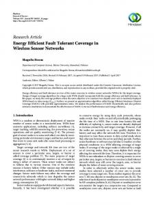
Figure 1: Reception probability of a 36 feet long wireless link for different moving window sizes. remaining battery energy.

The second part of the paper extends energy-efficient routing over multiple paths to increase network reliability under link failures. Figure 1 shows how the link quality between two Berkeley mica2dot [5] sensor nodes varies over time. The link quality at a distance greater than a certain value, which is 30f t in this case, shows similar behavior. Multipath routing can be used to provide robustness of the system against this kind of link failures. Multiple paths are discussed in [6] to rapidly find alternative paths between source and sink. The first to combine multiple path and minimum energy routing is [7]. The goal is to minimize the total energy consumed in forwarding each packet between a source The first part of this paper gives an LP formulation of the lifetime and a destination. However, the impact of this routing on netmaximization and approximates the LP solution by a sequence work lifetime is not considered. We introduce an algorithm to of least cost path calculation problems, in which the path cost is find multiple paths in order to maximize the network lifetime either the sum or the maximum of the cost of the nodes on that while increasing network resilience. path, and the cost of each node is a function of its initial and

Section 2 presents the background assumptions. Section 3 formulates the LP problem and gives the iterative algorithm. Section 4 discusses multiple path routing. Section 5 provides some concluding remarks.

Maximize t Subject to: fij >= 0 for i, j ∈ [1, N ] fij = 0 for (i, j) ∈ /E Σj fij − Σj fji = gi tt for i ∈ [2, N ] t(Σj ptx fij + Σj prx fji + ps gi + (1 − Σj fij − Σj fji )pl ) ∈ Ed and fij > 0. < j, i >∈ Ed for each (i, j) ∈ E. The iterative algorithm assigns Section 3.1 gives the LP formulation for optimal flow rates. Sec- a cost C to every link < i, j >∈ E and then finds shortest path ij d tion 3.2 gives iterative distributed algorithms that approximate tree from AP to all the nodes at the beginning of each time period the centralized LP solution. Simulations in section 3.3 show the to be used for routing until the end of that period. advantage of energy efficient routing over minimum hop routing. Since the cost of the links are used in finding the shortest path from AP to the sensor nodes, the cost of the directed link < 3.1 Linear Programming Formulation j, i >, Cji , is equal to the cost of including the node i on the path. The cost of node i at the p-th iteration is the ratio of the toThe variables in the optimization problem of Figure 2 are the packet flow rates fij , the average packet transmission time from i to j per unit time, and the network lifetime t. The objective is

3 Energy Efficient Single-Path Routing

power consumption 0.92mJ 0.69mJ 29.71mJ/sec 15µJ/sec 1.5µJ/sample

900

optimum lifetime non−optimum lifetime 800

700

600

network lifetime (day)

operation transmitting one packet receiving one packet listening to channel operating radio in sleep mode sampling sensor

Table 1: Power consumption in Berkeley mica nodes.

500

400

300

tal energy consumed up to period p over the total battery energy: 200

Ci =p∗

total energy consumed up to now = total battery energy

(1)

100

Σj ptx fij +Σj prx fji +ps gi +(1−Σj fij −Σj fji )pl . ei

(2)

0

10

20

30

40

number of nodes

Here fij is the average resulting flow rate on link < i, j >. Ci increases from 0 to 1 as network evolves. The link cost function can be any increasing function d, Cji = d(Ci ). For instance, the cost in [3] is the ratio of total battery energy to the remaining 1 energy, given by d(x) = 1−x . The next step is to calculate the shortest path tree from node 1 (AP) to all nodes. The cost of a path is either the sum of the costs of the links in the path for the least sum-cost path algorithm, or the maximum of the link costs for the least max-cost path algorithm. A Bellman-Ford procedure can be used to obtain the optimum tree for both algorithms.

3.3

Simulations

In the simulations, nodes are randomly distributed in a circular area of radius 100 units. The transmission range is slightly larger than that necessary for network connectivity [9]. There is an edge between the nodes closer than this transmission range. The results below are averages of the performance of ten different random configurations unless otherwise stated. The power consumption figures are in Table 1. The transmission rate is 50 kbps. The packet generation rate gi at each node i is 1/30 per second, which is a typical value for traffic monitoring [10]. The energy ei for all nodes except AP is for a pair of AA batteries, or 2200mAh at 3V. The sampling rate is 128Hz at each node.

Figure 3: Comparison of the lifetime for optimum and minimum hop routing. lems. The critical parameters are the type of least cost path algorithm, step interval and cost function. Step interval is the length of each iteration during which the same routing paths are used. Cost function emphasizes different battery levels at different intensities in least sum-cost path algorithm through the function d(x) in Section 3.2. Figure 4 shows the network lifetime for iterative algorithms. As the step interval increases, the lifetime of the network decreases because there are fewer iterations. For small step intervals, the lifetime is almost equal to the optimal for least max-cost path algorithm, and close to optimal for least sum-cost path algorithm with cost functions d(x) = x50 and d(x) = 1/(1 − x)50 . This suggests that for least sum-cost path, with d(x) = xn , n should not be too small since the cost becomes almost linear, making it hard to differentiate between a path having one node with small residual energy and many other nodes with high residual energy, and a path with many nodes with medium residual energy. Also, n should not so large that it is hard to differentiate between d(x) = xn values unless x is very close to 1. On the other hand, as n gets larger in d(x) = 1/(1 − x)n it gets closer to the optimal value since the path cost is close to the maximum of the link costs on the path.

Figure 3 compares the lifetime of the network using the optimal LP solution with minimum hop routing. The LP solution 4 Energy Efficient Multipath Routing increases network lifetime by 50-150 days. If energy spent in sampling were ignored in the lifetime calculations as in [3], the The goal of multipath routing is to increase the resilience of the LP solution would show further improvements. network against the failure of the links by trading off the energy consumption. The cost of a path p is the maximum of The distributed, iterative algorithms approximate the solution of the costs of the links in p whereas the cost of a set of paths LP formulation by iteratively solving minimum cost path prob-

700

Removing the arcs belonging to the shortest path in step 2 ensures that this path is not reproduced when the Bellman-Ford algorithm is run in the modified graph. Moreover, modifying the cost of the link in reverse direction permits the interlacing of the shortest path to be found in Step 4 with the one found in the original graph while eliminating the possibility of including the reverse link before removing the forward link. At the end of the algorithm, two disjoint paths are obtained by erasing the interlacing part of the two paths. Allowing for interlacing and the negativity of the links leads to optimality.

680

660

lifetime (day)

640

620

600

d(x)=x d(x)=x5 50 d(x)=x 500 d(x)=x 5000 d(x)=x d(x)=1/(1−x) d(x)=1/(1−x)5 50 d(x)=1/(1−x) d(x)=x,maxd LP

580

560

540

520

500 0 10

Minimum cost k edge-disjoint paths are generated iteratively from minimum cost k − 1 edge disjoint paths. The algorithm is similar to the 2 edge-disjoint path case: 1

2

10

10

3

10

step interval (hour)

Figure 4: Average battery lifetime of the random configurations of 20 nodes for different cost functions and step intervals.

1. For each < i, j > on the minimum cost k − 1 edge disjoint paths, remove the edge < i, j > and set the cost of the link < j, i > to Cji = −Cij . 2. Run Bellman-Ford algorithm to find the shortest path from the AP to node i in the resulting graph.

3. Remove the overlapping edges of the different paths. The P = {p1 , p2 , ..., pk } is the maximum of the cost of each path desired k paths results. in P . The minimum cost k link-disjoint path problem is: Given Gd = (V, Ed ), find a set of k link-disjoint paths P from node AP to a sensor node such that the cost of the set is minimized. We omit the proof of optimality of the algorithm.

4.1

Multiple Path Routing Algorithm

If node i has infinite cost in Step 2, then no more edge disjoint paths can be found. Then the algorithm stops before reaching k. An example of generating two edge-disjoint paths from AP to node 4 is given in Figure 5. The original network is given in Figure 5(a). The first path found is {AP, 2, 3, 4}, with the modified graph given in Figure 5(b). The next path found is {AP, 6, 7, 3, 2, 5, 4}. The two edge-disjoint paths resulting from the removal of the overlapping edges are then {AP, 2, 5, 4} and {AP, 6, 7, 3, 4}. Figure 5 (c) gives the modified graph as a result of these two paths. Since there is no path from AP to node 4 in this modified graph, no more edge-disjoint paths can be found.

The algorithm in [11] gives a minimum cost edge-disjoint path algorithm in an undirected graph where the cost of a path is the sum of its link costs. We modify this algorithm to find minimum cost edge-disjoint paths in Gd with the cost of a path being the maximum of its link costs based on the assumption that < i, j > and < j, i > are not disjoint links. Since nodes i and j transmit at the same power, links < i, j > and < j, i > both fail at the same time. Therefore, if one of them is used in a path, the other cannot be used in another path to provide edge disjoint multiple The algorithm is executed k times for each node. The runpaths. ning time of each iteration is dominated by Bellman Ford algoThis is the algorithm for minimum cost two edge-disjoint paths rithm. The2resulting running time of the algorithm is therefore O(k|E||V | ). from AP to a sensor node i:

The multipath routing can be implemented in a centralized man1. Run Bellman-Ford algorithm to find the shortest path from ner at the AP by running the above algorithm for each node after AP to the sensor node i in Gd . collecting the topology information and then disseminating this information to the nodes. The algorithm can be made distributed 2. For each < i, j > on the shortest path, remove the edge by running a distributed Bellman-Ford algorithm for each path < i, j > and set the cost of the link < j, i > to Cji = −Cij . updating the link cost according to the previous paths found. 3. Run Bellman-Ford algorithm to find the shortest path from Bellman-Ford algorithm takes |V | pulses for each path so k|V | pulses to generate k edge-disjoint paths to each node. the AP to node i in the modified graph. 4. Remove the overlapping edges of the two paths. The desired pair of paths results.

5

1

1

4

0

3

2 2

0 6

1

AP

4

1

4

3

1

3

2

-1

2

1

1

4

95

3

2

AP

100

5 3

2

1 0 6

7

4

1

1

1

(a)

(b)

1 7

5 -4 2

AP -1

2

-3 3

4 -3

1

90

-3

-2

85

percentage of nodes

4

80

75

70

65

d(x)=x,p=0.1 d(x)=x,p=0.2 d(x)=x,p=0.3 d(x)=1,p=0.1 d(x)=1,p=0.2 d(x)=1,p=0.3

-2 60

-1 6

7 -1 (c)

55

50

Figure 5: (a) Original graph Gd = (V, Ed ). (b) Modified graph after finding the path {AP, 2, 3, 4}. (c) Modified graph after finding the paths {AP, 2, 5, 4} and {AP, 6, 7, 3, 4}.

4.2

1

1.5

2

2.5

3

3.5

4

4.5

5

5.5

6

number of paths

Figure 6: Average percentage of the nodes that can send their packets successfully to the AP for a random 20-node network.

Simulations

because the nodes may not find another edge-disjoint path afThe simulations help to understand the tradeoff between the re- ter choosing minimum cost paths, thereby preventing the load of silience of the network to link failures and the extra energy con- critical nodes from increasing linearly with the number of multiple paths. The same kind of behavior is observed for the simulasumption. tions of different number of nodes in the number of successfully Figure 6 shows the average percentage of the nodes that can received packets and the lifetime as a result of multipath routing. send their packets successfully to the AP for different link fail- The only difference is that the percentage of the successful nodes ure probabilities, p, for a random 20-node network. The cost decreases as the number of nodes increases since the number of d(x) = x corresponds to minimizing the maximum cost on hops to reach AP increases. the k disjoint paths for the cost defined in Section 3.2 whereas d(x) = 1 corresponds to choosing any k disjoint paths without considering the real costs. The percentage of the successful 5 Conclusion nodes increases by 15 − 30% for both cases. The rate of increase decreases with the number of paths since no more paths can be found for the nodes (The average number of paths found In this paper, we present a routing protocol for sensor networks, for the nodes are 1, 1.8421, 2.6316, 3.2632, 3.8947, 4.4211 for in which all data packets are destined for a single collection node, 1, 2, 3, 4, 5, 6 paths respectively). The d(x) = 1 case gives with the goal of maximizing the time duration until the first node slightly better result since the total number of edges in the least dies. cost paths for d(x) = x may be larger than that for d(x) = 1. We first focus on single path routing. We formulate the path opFigure 7 shows the average percentage of the lifetime that can timization as a Linear Programming (LP) problem in which the be achieved at different multiple paths for a random 20-node net- objective is to maximize the lifetime of the network. This optimal work. Since the edge-disjoint multiple paths between a sensor routing is shown to increase the network lifetime by 50-150 days node and the AP can contain common nodes, we consider two over the minimum hop routing. We then describe a distributed alcases: join and no join. The join case assumes that a node com- gorithm based on iterative least cost path routing where the cost mon to multiple paths for the same source-destination pairs waits of each path is either the sum or the maximum of the cost of until it receives the same packet over multiple paths and then the nodes on that path at each step. The distributed algorithm is sends it only once whereas no join case assumes that they are extended to include multiple paths between each source and destransmitted separately. The d(x) = x cost increases the network tination in the network to provide the resiliency of the network lifetime by 20% over the d(x) = 1 cost. Moreover, the lifetime to link failures. We introduce a multipath routing algorithm that only decreases by 50% for 6 multiple paths, where an average is optimal in terms of minimizing the maximum cost on the mulof 4.4211 paths are found for each node. This slow decrease is tiple paths from each sensor node to the AP. We show that the

100

[8] Swetha Narayanaswamy, Vikas Kawadia, R. S. Sreenivas, and P. R. Kumar, Power control in Ad hoc networks: theory, architecture, algorithm and implementation of the COMPOW protocol, Proceedings of European Wireless 2002, February 2002, Italy.

d(x)=x,join d(x)=x,no join d(x)=1,join d(x)=1,no join

90

percentage of optimum lifetime

80

70

[9] B. Krishnamachari, S. B. Wicker, and B. Bejar, Phase transition phenomena in wireless ad hoc networks, Symposium on Ad-Hoc Wireless Networks, GlobeCom 2001, San Antonio, Texas, November 2001.

60

50

[10] S. Coleri, PEDAMACS: Power efficient and delay aware medium access protocol for sensor networks, MS Thesis, Department of Electrical Engineering and Computer Science, University of California, Berkeley, December 2002.

40

30

20

1

1.5

2

2.5

3

3.5

4

4.5

5

5.5

6

number of paths

Figure 7: Percentage of optimal lifetime that can be achieved at different multiple paths for a random 20-node network. number of successfully received packets at the AP increases by 20% for a decrease of 50% in the resulting lifetime of the network.

References [1] E. M. Royer, and C. Toh, A review of current routing protocols for ad hoc mobile wireless networks, IEEE Personal Communications, pp. 46-55, April 1999. [2] S. Singh, M. Woo, and C. Raghavendra, Power-aware routing in mobile ad hoc networks, MOBICOM 1998, pp.181190. [3] J-H. Chang and L. Tassiulas, Energy conserving routing in wireless ad hoc networks, IEEE INFOCOM 2000, vol. 1, pp. 22-31. [4] M. Bhardwaj and A. P. Chandrakasan, Bounding the lifetime of sensor networks via optimal role assignments, IEEE INFOCOM 2002, pp.1587-1596. [5] www.tinyos.net [6] D. Ganesan, R. Govindan, S. Shenker and D. Estrin, Highly-resilient, energy efficient multipath routing in wireless sensor networks, Mobile Computing and Communications Review, vol. 4, no. 5, October 2001. [7] A. Srinivas and E. Modiano, Minimum energy disjoint path routing in wireless ad hoc networks, ACM MOBICOM 2003.

[11] R. Bhandari, Optimal physical diversity algorithms and survivable networks, IEEE Symposium on Computers and Communications, July 1997, pp.433-441