65â77,. 1982. Fault Tolerant Operation of Kinematically. Redundant Manipulators for Locked. Joint Failures. Christopher L. Lewis and Anthony A. Maciejewski.
622
IEEE TRANSACTIONS ON ROBOTICS AND AUTOMATION, VOL. 13, NO. 4, AUGUST 1997
have compared this result to a naive counting argument and found that the counting argument erroneously predicts that only two fingers are needed for planar symmetric full rank mappings. We have found that, for spatial workparts, a five-fingered grasp allows for the maximum range of attainable matrices. However, there remains one restriction on the attainable workpart damping matrices that persists regardless of the number of fingers that grasp the workpart or where they grasp it. By examining the left nullspace of B ; we are able to characterize the restrictions on attainable workpart damping matrices when a workpart is grasped with an insufficient number of fingers to achieve a full rank mapping. Examination of B reveals that the circulant matrix describes the fundamental restriction on all damping matrices attainable by spatial workparts.
[19] S. Vougioukas and S. Gottschlich, “Automatic synthesis and validation of compliance mappings,” in Int. Conf. Robot. Automat., Atlanta, GA, 1993, pp. 491–496. [20] D. E. Whitney, “Quasistatic assembly of compliantly supported rigid parts,” ASME J. Dynam. Syst., Measure., Contr., vol. 104, pp. 65–77, 1982.
REFERENCES
Abstract—This paper studies the degree to which the kinematic redundancy of a manipulator may be utilized for failure tolerance. A redundant manipulator is considered to be fault tolerant with respect to a given task if it is guaranteed to be capable of performing the task after any one of its joints has failed and is locked in place. A method is developed for determining the necessary constraints which insure the failure tolerance of a kinematically redundant manipulator with respect to a given critical task. This method is based on estimating the bounding boxes enclosing the self-motion manifolds for a given set of critical task points. The intersection of these bounding boxes provides a set of artificial joint limits that may guarantee the reachability of the task points after a joint failure. An algorithm for dealing with the special case of 2-D self-motion surfaces is presented. These techniques are illustrated on a PUMA 560 that is used for a 3-D Cartesian positioning task.
[1] D. S. Ahn, H. S. Cho, K. Ide, F. Miyazaki, and S. Arimoto, “Strategy generation and skill acquisition for automated robotic assembly task,” in Proc. IEEE Int. Conf. Robot. Automat., Arlington, VA, 1991, pp. 128–133. [2] M. Cutkosky and I. Kao, “Computing and controlling the compliance of a robotic hand,” IEEE Trans. Robot. Automat., vol. 5, pp. 151–165, 1989. [3] V. Gullapalli, R. A. Grupen, and A. G. Barto, “Learning reactive admittance control,” in IEEE Int. Conf. Robot. Automat., Nice, France, 1992, pp. 1475–1480. [4] J. Kerr and B. Roth, “Analysis of multifingered hands,” IJRR, vol. 4, no. 4, pp. 3–17, 1986. [5] V. Kumar and K. J. Waldron, “Suboptimal algorithms for force distribution in multifingered grippers,” IEEE Trans. Robot. Automat., vol. 5, pp. 491–497, 1989. [6] Z. Li, P. Hsu, and S. Sastry, “Grasping and coordinated manipulation by a multifingered robot hand,” IJRR, vol. 8, no. 4, pp. 33–50, 1989. [7] Z. Li and S. Sastry, “Task-oriented optimal grasping by multifingered robotic hands,” IEEE Trans. Robot. Automat., vol. 4, pp. 33–44, 1988. [8] T. Lozano-Perez, “Motion planning for simple robot manipulators,” in Third Int. Symp. Robot. Res., Paris, France, 1985, pp. 133–140. [9] T. Lozano-Perez, M. T. Mason, and R. H. Taylor, “Automatic synthesis of fine-motion strategies for robots,” IJRR, vol. 3, no. 1, pp. 3–24, 1984. [10] S. Lui and H. Asada, “Teaching and learning of deburring robots using neural networks,” in IEEE Int. Conf. Robot. Automat., Atlanta, GA, 1993, pp. 339–345. [11] C. Melchiorri, “Static force analysis for general cooperating manipulators,” in IEEE Int. Conf. Robot. Automat., San Diego, CA, 1994, pp. 888–893. [12] Y. Park and G. Starr, “Optimal grasping using a multifingered robot hand,” in IEEE Int. Conf. Robot. Automat., Cincinnati, OH, 1990, pp. 698–694. [13] S. Payandeh and A. Goldenberg, “Grasp impedance: Examples of finger’s targeted impedance,” in Proc. Third Int. Conf. Intell. Contr., Arlington, VA, 1989, pp. 479–483. [14] M. A. Peshkin, “Programmed compliance for error-corrective assembly,” IEEE Trans. Robot. Automat., vol. 6, pp. 473–482, 1990. [15] J. Ponce, S. Sullivan, J. D. Bossionnat, and J. P. Merlet, “On characterizing and computing three- and four-finger force closure grasps of polyhedral objects,” in IEEE Conf. Robot. Automat., Atlanta, GA, 1993, pp. 821–827. [16] J. K. Salisbury and M. T. Mason, Robot Hands and the Mechanics of Manipulation, P. H. Winston and M. Brady, Eds. Cambridge, MA: The MIT Press (Series in Artificial Intelligence), 1985. [17] J. M. Schimmels and M. A. Peshkin, “Synthesis and validation of non-diagonal accommodation matrices for error-corrective assembly,” in Proc. IEEE Int. Conf. Robot. Automat., Cincinati, OH, 1990, pp. 714–719 [18] J. C. Trinkle, P. F. Stiller, and A. O. Farahat, “Second-order stability cells of a frictionless rigid body grasped by rigid fingers,” in IEEE Int. Conf. Robot. Automat., San Diego, CA, 1994, pp. 2815–2821.
Fault Tolerant Operation of Kinematically Redundant Manipulators for Locked Joint Failures Christopher L. Lewis and Anthony A. Maciejewski
Index Terms—Fault tolerance, Jacobian matrices, kinematically redundant, manipulator kinematics, manipulators, redundant systems.
I. INTRODUCTION Kinematically redundant manipulators have been proposed for use in the cleanup and remediation of nuclear and hazardous materials, as well as for remote applications such as space or sea exploration [1], [2]. In these applications repairing broken actuators and sensors is impossible and the probability of their failure is increased due to the harsh operating environment [3]–[5]. The redundant degrees of freedom may or may not also be equipped with redundant actuators [6]. The extra degrees of freedom (DOF) of a redundant manipulator may be used to compensate for a failed joint if the manipulator has been properly designed and controlled. The most basic task of a manipulator, i.e., the positioning and/or orienting of the end-effector in the workspace, is described by the forward kinematic equation x = f (�)
(1)
where x 2 Rm is the generalized vector of the position and/or orientation of the end-effector and � 2 Rn is the vector of joint
Manuscript received July 1, 1994; revised April 29, 1996. This work was supported by Sandia National Laboratories under Contract 18-4379B and Contract AL-3011, and by the National Science Foundation by Grant CDR 8803017 to the Engineering Research Center for Intelligent Manufacturing Systems. An earlier version of this paper was presented at the 1994 IEEE International Conference on Robotics and Automation. This paper was recommended for publication by Associate Editor V. Kumar and Editor A. Goldenberg upon evaluation of the reviewers’ comments. C. L. Lewis is with Sandia National Laboratories, Albuquerque, NM 87185 USA. A. A. Maciejewski is with the School of Electrical and Computer Engineering, Purdue University, West Lafayette, IN 47907 USA. Publisher Item Identifier S 1042-296X(97)03815-9.
1042–296X/97$10.00 1997 IEEE
IEEE TRANSACTIONS ON ROBOTICS AND AUTOMATION, VOL. 13, NO. 4, AUGUST 1997
623
variables. In this framework, point-to-point tasks can be described by a series of end-effector positions and/or orientations to be obtained at desired times, i.e., x(ti ), with an inverse kinematic function � = f 01 (x)
(2)
being used to determine the corresponding required joint values �(ti ). A kinematically redundant manipulator can, in general, satisfy an endeffector positioning and/or orienting task x(ti ) with an infinite family of joint values satisfying (1). The underlying premise for advocating the use of redundant manipulators for critical applications is that if a joint should fail, then the redundancy of the manipulator may still permit completion of the task. In this work, it is assumed that failed joints are locked in a known position. The immobilization of a joint may be directly due to the failure itself, the indirect result of a very high gear ratio on an actuator that has lost power, or due to brakes that have been applied by failure detection software [7] (e.g., Robotics Research Corporation manipulator). If failed joints are locked individually then a single joint failure reduces the number of degrees of freedom of the system by one. The new inverse kinematic function f^01 differs markedly from the original one, and the resulting system may or may not be capable of completing the given task x(ti ). In [8] a method is described for designing manipulators to be fault tolerant with regard to a given point-to-point task. The authors assume that any joint may fail anywhere within its entire range of motion. A manipulator is said to be fault tolerant with respect to a given set of task points x(ti ) only if there exist solutions to (1) for every possible failure in all joint configurations. With this assumption, the worst case typically occurs when a failing joint is folded in on itself. In contrast, the approach presented here achieves failure tolerance by imposing constraints on the motion of all joints prior to a failure. By judiciously selecting specific solutions which satisfy these constraints from the family of solutions to (1), the worst case need not occur. Thus failure tolerance may be achieved with less complex manipulator designs and for manipulators not originally designed with failure tolerance in mind. A somewhat different, but related, measure of failure tolerance for redundant manipulators was presented in [9]. The focus of this work was to guarantee a maximum amount of dexterity in the vicinity of a failure by controlling the configuration of the robot in anticipation of a failure. This type of failure tolerance is particularly suited for tasks described by a desired end-effector velocity as opposed to those described by discrete positions and/or orientations. At the velocity level, the kinematic equations relating the joint rates �_ to the end-effector’s velocity x_ are given by
2n
x_ = J �_
(3)
is the manipulator Jacobian matrix which is a where J 2 R function of the manipulator’s configuration. The solution for all joint rates that satisfy the desired end-effector velocity can be represented by m
�_ = J + x_ + (I
0 J + J )z (4) + indicates the pseudoinverse, (I 0 J J ) is the projection
where + onto the null space, and z represents an arbitrary vector in the joint velocity space [10]. The second term in this equation indicates that there is a family of joint trajectories that satisfy (3). However, unlike the kinematic function f relating the joint values to the end-effector’s position and/or orientations, the Jacobian for the failed system is easily derived from the original system’s Jacobian by zeroing the column of the failed joint. Using this fact [9] develops an inverse kinematic function which insures that the manipulator will have the maximum amount of local dexterity after an arbitrary joint failure. The measure of dexterity in
Fig. 1. A three degree-of-freedom planar manipulator with equal link lengths is shown with the curves in the workspace having maximum and minimum failure tolerance capabilities. The points A; B , and C are representative task space points that are analyzed for their global failure tolerance properties.
this case is defined as the smallest singular value of the Jacobian �m so that a local kinematic failure tolerance measure kf m is given by kf m(�) = min �m (i J )
=1ton
i
(5)
where i J is the manipulator Jacobian matrix for the system with its ith joint locked. It is important to note that since the units of the manipulator Jacobian are not homogeneous an appropriate scaling of the rows associated with the linear components must be performed before this measure is meaningful [11], [12]. The value of kf m is a worst-case measure of how much the nonfailed joints must increase their velocity in order to compensate for the loss of end-effector velocity due to the failed joint. A larger value of kf m will require smaller discontinuous increases in the operating joints, thus resulting in smaller transients in the end-effector tracking error. Unfortunately, this measure is inherently local in nature and can not guarantee that the complete trajectory remains feasible after the failure. To address this more global issue, this paper discusses techniques for determining constraints on each joint’s motion which guarantee the failure tolerance of the entire task. The constraints determined by this method are upper and lower bounds on the range of motion for each joint and thus will only affect the motion of the manipulator when it is operating near these software joint limits. Therefore, it is still possible to utilize the redundancy to maximize the remaining local dexterity after a joint failure by maximizing kf m [9]. An inverse kinematic solution that optimizes kf m under the constraint of maintaining the specified software joint limits is thus able to guarantee that the desired task can be completed, as well as minimize the transient effects of the joint failure. The remainder of this paper is organized as follows. First, a method for analyzing the fault tolerance of a given position and/or orientation in the workspace is discussed. Second, the constraints necessary to guarantee fault tolerance for a single task point are described. Then, a method for determining the constraints necessary to guarantee the fault tolerance of the manipulator with respect to the given task described by a sequence of critical points is outlined. Finally, these techniques are illustrated using a PUMA 560 manipulator to perform a 3-D Cartesian positioning task. II. SURFACES
OF
SELF-MOTION
For a kinematically redundant manipulator the family of joint configurations satisfying (1) forms an (n 0 m)-dimensional hypersurface in the n-dimensional configuration space of the manipulator [13], [14]. Joint motion constrained to this hyper-surface does not affect the position and/or orientation of the end-effector so that these
624
IEEE TRANSACTIONS ON ROBOTICS AND AUTOMATION, VOL. 13, NO. 4, AUGUST 1997
Fig. 2. The set of joint configurations that keep the manipulator’s end-effector at a single 2-D position form curves in the configuration space of the manipulator. The curves shown are the self-motion curves for the 3 link planar manipulator depicted in Fig. 1. The self-motion curves for some regions of the workspace are markedly larger than others. Points with large self-motion curves tend to be more failure tolerant.
hyper-surfaces are frequently referred to as self-motion manifolds. The null space of the manipulator’s Jacobian given by the set of vectors satisfying (3) with x_ = 0 defines the tangent hyperplane to the self-motion manifold. As a simple example, consider the 3 DOF planar manipulator shown in Fig. 1 for which the self-motion manifolds are 1-D curves. For this manipulator a projection of the self-motion curves onto the (�2 ,�3 ) plane is shown in Fig. 2. Each curve represents the family of joint variable combinations which place the end-effector at a constant radius from the base. From the figure, one can see that some regions of the workspace have larger self-motion manifolds than others. For instance, consider the points corresponding to the reach singularity which occur when the arm is fully extended and the end-effector is at the boundary of its workspace. Each of these points is reachable in only a single joint configuration which corresponds to the self-motion manifold also being a point. Obviously, a workspace boundary point may not be reachable after any joint failure unless the failure occurs with the end-effector at that point. In contrast, the workspace points exactly one link length from the base have self-motion manifolds which span the entire range of joint values for all three joints. In this unique case the failed manipulator will always be able to reach the entire set of points one link length from the base regardless of which joint fails, or the configuration in which it fails. This family of points is in fact the single joint failure tolerant workspace for this manipulator. A critical task consisting of points which lie solely in this family may be completed regardless of any single failure. It is now possible to state a key point of this paper. To guarantee that a manipulator is capable of returning to a critical workspace position and/or orientation x(ti ), the motion range for each of the n joints must be constrained to lie within the range spanned by the self-motion manifold associated with that position and/or orientation. The minimum and maximum joint values of the ith joint, denoted �i and �i , respectively, can be determined from the minimum
and maximum values of �i over the entire self-motion manifold. This effectively superscribes an n-dimensional bounding box aligned with the joint axes around the self-motion manifold. It is important to note that these joint restrictions are implemented as simple software joint limits and that after a joint failure they can be removed. The size of the self-motion manifold bounding box is a measure of the inherent failure tolerance of the workspace position and/or orientation for which it was computed. If the manipulator fails while operating within the bounding box of a given desired end-effector position and/or orientation x3 , then it will always be able to position and/or orient its end-effector at x3 regardless of where the end-effector is when the failure occurs. As a specific example, consider again the 3 DOF manipulator for which the bounding boxes associated with the self-motion surfaces for the three workspace points labeled A; B , and C in Fig. 1 have been drawn in Fig. 2. Note that although �1 and its associated boundaries are not shown, they also need to be considered. If we want to guarantee that task point A is reachable after any single joint failure, the joint values must be restricted to the range of the bounding box for A’s associated self-motion manifold. Now, if in addition we want to guarantee that task point B is reachable after any single joint failure, the joint values must be further restricted to B’s bounding box (which is the intersection of boxes A and B). Note that by doing so we have restricted allowable configurations for being at task point A to only those inside of B’s bounding box. This family of configurations is represented by the two small curves at the upper right and lower left corners of B’s bounding box in Fig. 2. Notice that if the manipulator is in a configuration near the center of bounding box B when a joint failure occurs, then the artificial joint restrictions must be released for the manipulator to reach task point A. Finally, consider trying to add task point C to this scenario. The intersection of the three bounding boxes is indicated with a bold line in Fig. 2. By design if a joint fails while operating in this region then by relaxing these artificial joint limits, the manipulator can reach all three task points. However, with these artificial joint restrictions in place, the family of configurations for point A has been reduced to only the curve in the upper right corner of the bold box. The family of configurations for point B has been reduced to a single point at the lower left corner of the bold box. Unfortunately, none of task point C’s self-motion manifold lies within the bold box and therefore it is unreachable with these artificial constraints in place. Constraining the motion of a manipulator’s joints prior to a failure will, in general, render a significant portion of the original workspace unreachable. However, these joint restrictions are crucial for eliminating the possibility of a joint failing in a catastrophic configuration, i.e., one which precludes reaching a critical workspace position and/or orientation. Thus, while it may appear counterintuitive, imposing appropriate software joint limits prior to a failure can actually increase the size of the workspace that can be guaranteed reachable after an arbitrary failure. Fig. 3 illustrates this point using the simple 3 DOF manipulator from Fig. 1. Evaluating the resulting workspaces after all possible joint failures and intersecting these regions with the original constrained workspace results in the guaranteed failure tolerant workspace. This represents the portion of the workspace in which any path can be tracked both before and after any joint failure. Thus the penalty for requiring failure tolerance is an approximately 60% reduction in the workspace. Note that the original unconstrained failure tolerant workspace in Fig. 1 consisted of only a circle having a one link length radius. III. JOINT CONSTRAINTS
TO
GUARANTEE FAULT TOLERANCE
As was indicated in the previous section, a workspace position and/or orientation x3 may be guaranteed to be reachable regardless
IEEE TRANSACTIONS ON ROBOTICS AND AUTOMATION, VOL. 13, NO. 4, AUGUST 1997
625
Fig. 3. Restricting the range of motion of each joint yields a reduced workspace. However, restrictions can eliminate the possibility that a joint will fail in a configuration where the partially failed system is unable to reach critical regions of the workspace. The workspace of the 3 DOF planar manipulator described in Fig. 1 is shown in the upper left. The workspace that remains reachable to the system under the joint limit constraints indicated is shown in the upper right. The central figures depict the regions guaranteed to be reachable regardless of where within the restricted range each joint fails. The combined intersection of the restricted workspace and each of the three failure reachable regions is the failure tolerant workspace. The bottom figure indicates the failure tolerant workspace for this manipulator with these constraints.
Fig. 4. A linearly increasing spiral passes within a controlled distance from every point in the plane and thus it may be used to estimate the bounds of a 2-D surface in an n-dimensional space.
of joint failures if the manipulator is constrained to operate within the associated self-motion manifold’s bounding box. This is evident since regardless of which joint fails, by definition, there must exist at least
one alternative configuration on the self-motion manifold associated with x3 that corresponds to the joint value at which the joint failed. Therefore, the problem of maintaining the fault tolerance of a given critical position and/or orientation reduces to that of maintaining joint limits specified by the bounding box of the self-motion manifold for that position and/or orientation. An effective technique for avoiding joint limits is to use (4) and select z to result in motion away from the joint limits [10], [14]. The vector z may be computed by combining smooth functions so that this term only affects the manipulator’s motion when it is near the joint limit [15]. For fault tolerance it is advantageous to locate critical task points in positions and/or orientations where the self-motion manifold bounds are large. One example of designing around a critical task point is that of a mobile robotic platform for disposing of unexploded ordinance. In this case the depository for the explosives would be the critical task point to be located on the platform. Such critical points should not generally be placed near the manipulator workspace boundaries since joint failures will render such regions unreachable. Although computationally intensive, the chore of measuring the size of the self-motion manifolds throughout the workspace can be performed off-line. It was also shown that imposing constraints on the range of motion of each joint prior to a failure can result in entire regions of the workspace that are failure tolerant. However, determining adequate constraints and the resulting fault tolerant workspace for a general redundant manipulator is computationally difficult. Fortunately, insuring the failure tolerance of a specific task is more tractable. To insure that a specific task defined by a sequence of points may be performed regardless of joint failures, each point is
626
IEEE TRANSACTIONS ON ROBOTICS AND AUTOMATION, VOL. 13, NO. 4, AUGUST 1997
a controlled distance from every point in the plane, when it is transformed onto the self-motion surface it will tend to fill the surface. An iterative transformation procedure from parameter to configuration space is given by
�_
Fig. 5. For a 3-D Cartesian positioning task the PUMA has two redundant degrees of freedom. Therefore it has the freedom to move its joints while holding the position of its end-effector stationary. The spiral gives an indication of the 2-D surface embedded in the 5-D configuration space that describes how the first five joints of a PUMA can be moved without changing the 3-D Cartesian position of the end-effector.
analyzed, the associated range of its self-motion surface determined, and then the intersection of the ranges over all points is determined in order to identify the required joint constraints. Then, as was pointed out in the example illustrated with Figs. 1 and 2, it must be verified that the manipulator is able to reach each critical point while maintaining the constraints. Once this is done, then simply imposing the resulting constraints allows the manipulator to execute the task in a fault tolerant manner. In summary, the following procedure is used to guarantee the failure tolerance of a redundant manipulator with respect to critical tasks. First, the workspace is analyzed to find regions having large self-motion manifolds. Second, critical tasks are placed in these regions of the workspace. Third, the bounding boxes for the self-motion surfaces associated with each critical position and/or orientation are determined. Fourth, the intersection of the bounding boxes is calculated to determine the required constraints. Fifth, each critical workspace point is checked to determine if the manipulator is capable of positioning and/or orienting its end-effector at the desired position and/or orientation while maintaining the constraints imposed by the intersection of all bounding boxes. Finally, (4) is used with a combination of joint limit avoidance and kf m optimization to insure both the reachability of all specified task points and maximum dexterity in the vicinity of the failure. IV. ESTIMATING SELF-MOTION MANIFOLDS It has been shown that the global fault tolerance associated with a position and/or orientation in the workspace is characterized by the self-motion manifold of the manipulator when its end-effector is at that position and/or orientation. Several iterative methods exist in the literature for characterizing 1-D self-motion curves [13], [16]–[18]. For a 2-D self-motion surface, a simple and effective method for estimating the bounds of the self-motion surface is to iteratively trace out a linearly increasing spiral on the self-motion surface. Keeping track of the values obtained by each joint along the spiral provides an estimate of the bounding box containing the self-motion surface. A 2-D nonescaping spiral parameterized by the polar coordinates � and r, depicted in Fig. 4, has the form
�_ r
= =
v r
�
(6)
where v is the speed along the spiral and controls the distance between successive rotations. Since this particular spiral passes within
+ 3 0 x)
vn + J (x = sin(�)^ vn01 + cos(�)^
(7)
where v^n01 and v^n are orthogonal unit vectors that span the null space of the manipulator’s Jacobian evaluated at the current configuration. The vectors v^n and v^n01 can be computed as the singular vectors from the singular value decomposition of J . Since v^n01 and v^n are not unique, one must be careful to insure that the vectors chosen are the ones nearest to those of the previous iteration. For example, if the current singular vectors are represented by v^n01 and v^n then once (7) is evaluated and used to update the manipulator configuration, the new Jacobian will in general have different singular vectors v^n0 01 and v^n0 . To accurately reflect the continuous rotation of these two vectors as the tangent plane rotates, one can use the following set of equations
v^n01 v^n
= =
where
�=
(1
�w ^1
+
0 �)w^1 0
(1
0 �)w^2 �w ^2
T^ 2 (w ^1 v n01 ) T T 2 (w ^ v ^n01 ) + (w ^ v ^n01 )2
1
2
(8)
(9)
^1 and w ^2 are any unit vectors that span the new null space. and w Note that the sign should be examined to select the smallest resulting rotation. An ideal algorithm for computing the SVD that automatically calculates the continuous rotation of the null space is presented in [19]. An illustration of this technique for mapping out a 2-D self-motion surface is presented in Fig. 5. This figure shows a 3D projection of the 5-D configuration space for a PUMA used in 3-D Cartesian positioning tasks. For systems with more than two degrees of redundancy, an estimate of the size of the self-motion manifold may be obtained using a Jacobian iteration of the form
ei + J + (x3 0 x) �_ = 6(I 0 J + J )^
(10)
where e^i is a unit vector along the ith joint axis and the error term x3 0 x is the difference between the desired end-effector position and/or orientation and its actual position and/or orientation. In practice, the first term provides motion along the self-motion manifold until the tangent hyperplane of the self-motion manifold becomes orthogonal to the joint axis direction e^i , while the second term eliminates errors that could have accumulated during the iterative procedure [17]. Since this technique is effectively a local optimization, it is subject to being trapped by local extrema and may provide suboptimal estimates of a bounding box. On the other hand, these two methods guarantee that the computed bounding box does not contain disjoint manifolds. V. AN EXAMPLE USING
A
PUMA
To demonstrate the concepts outlined above, a failure tolerance analysis was performed on a PUMA 560 manipulator for an example 3-D Cartesian positioning task. The Denavit and Hartenberg parameters for the system are given in Table I. Since the sixth joint of the PUMA only rotates the end-effector and does not change its Cartesian position, the manipulator has nominally two redundant degrees of freedom with respect to the task space. Note that this is only true for tool points that are collinear with the sixth joint axis. A simple Cartesian positioning task defined by five points was chosen as an illustrative example (see Fig. 6). Following the basic design procedure outlined in the previous section, the task was first
IEEE TRANSACTIONS ON ROBOTICS AND AUTOMATION, VOL. 13, NO. 4, AUGUST 1997
627
Fig. 6. A simple Cartesian positioning task is used to demonstrate the failure tolerance of a PUMA 560 manipulator.
TABLE I PUMA 560 DH PARAMETERS
Fig. 8. Some locations in the PUMA’s workspace allow for wider variations in the joints than others. With the end-effector’s Cartesian position fixed at a given location the range of motion for each joint may be determined using the projected spiral technique shown in Fig. 5. Here, two distinct workspace points are shown, one having a large self-motion surface and one with a small one, as indicated by their bounding boxes.
TABLE II SELF-MOTION SURFACE BOUNDARY DATA
Fig. 7. Positioning a critical task in regions having a high degree of failure tolerance insures that the task can be executed regardless of joint failures. In this example the optimal Cartesian position of task point P 1 is determined by calculating the volume of the self-motion surface bounding box as a function of the distance from the PUMA’s first joint axis. This is a 1-D optimization since the height of point P 1 is constrained to be 0.5 m and the volumes are independent of the first joint axis as long as joint limits are not reached. The discontinuities in this function are expected due to changes in the topology of the self-motion manifolds.
optimally positioned within the workspace. In general, one would perform a search over the entire workspace, however, for this example the search for the optimal task placement was constrained since the box was required to rest on a table in front of the PUMA. This required that the point P 1 be at a height of 0.5 m. We decided to optimally locate the point P 1 since it was the closest task point to the centroid of all task points. Alternatively, one could optimize a measure that consisted of the weighted sum of the size of the self-motion surfaces over all task points. In our case the size of the self-motion manifold is independent of the first joint angle so
the search for the optimal task placement was only a function of the distance from the first joint axis. A plot of the volume of the self-motion manifold bounding boxes as a function of the distance between the first joint axis and the end effector at a height of 0.5 m is shown in Fig. 7. The task was thus placed so that P 1 was located a distance of 0.9 m from the first joint axis since this provided maximum failure tolerance for this task point. Note that the volume of the self-motion bounding box can be ill-defined if the manipulator possesses a mix of rotational and prismatic joints. In this case, to
628
IEEE TRANSACTIONS ON ROBOTICS AND AUTOMATION, VOL. 13, NO. 4, AUGUST 1997
Fig. 9. PUMA with its end-effector at the critical point in an optimal pose. Fig. 11. PUMA with its end-effector moved from the nonfault tolerant configuration to its closest approach to the critical point after the first joint has failed.
Fig. 10. PUMA with its end-effector at a point far away from the critical point in a configuration that was obtained without considering fault tolerance. Should a joint fail, it will not be able to position its end-effector at the critical point.
provide a unitless measure one can divide each axis of the bounding box by the range of its corresponding joint. The self-motion surfaces for each of the five points were then examined using the spiral procedure outlined in Section IV. The resulting bounding box data is presented in Table II. To illustrate the benefits of using the self-motion manifold’s volume for task placement, Fig. 8 displays the bounding box for the optimal point P 1 along with a representative Cartesian position that has a very poor measure of failure tolerance. If P 1 had been placed at a position with such a poor degree of fault tolerance then the task would not have been completable in a failure tolerant manner due to a null intersection of the self-motion manifold bounding boxes. Next, with the motion of the joints constrained to lie within the combined intersection of the bounding boxes for all the points, it was verified that each point could be reached by iteratively solving (4) with the desired velocity being approximated by a position error until a solution was found. Furthermore, within these joint constraints
Fig. 12. PUMA with its end-effector at the same point as in Fig. 10 but in a configuration within the bounds of the self-motion surface’s bounding box associated with the critical point. Regardless of which joint fails in this configuration, it will be able to reposition its end-effector at the critical point.
the local measure of failure tolerance kfm is optimized to arrive at a unique configuration, an example of which is shown in Fig. 9. Now, with the constraints imposed, the manipulator is considered to be failure tolerant with respect to this task. To verify this (4) was implemented to trace out the trajectory through the points. Then, the technique was tested by simulating joint failures at random time intervals by locking a single joint. As expected, the manipulator was always able to complete the desired task. To further demonstrate the advantages of performing the above analysis, consider the point P 1 to be a critical workspace Cartesian position, e.g., a tool rest, which the manipulator must reach even after a joint failure. First, the manipulator was moved to a point far away from the critical point without considering the effects of the joint failure constraints. This configuration is shown in Fig. 10. The
IEEE TRANSACTIONS ON ROBOTICS AND AUTOMATION, VOL. 13, NO. 4, AUGUST 1997
629
REFERENCES
Fig. 13. PUMA with its end-effector moved from the failure tolerant configuration at the far point to the critical point while its first joint is locked. This demonstrates the failure tolerance of the configuration in Fig. 12 with respect to this critical point.
first joint was then locked and the manipulator attempted to move to P 1. It could not reach P 1, but the configuration having the minimum position error is shown in Fig. 11. Next, using the bounding box of the self-motion surface for the point P 1, joint limits were imposed to guarantee the failure tolerance of the manipulator with respect to this position. Then, with the constraints imposed, the manipulator is moved back to the same far away point. The configuration is quite different from before (see Fig. 12) and it has the property that regardless of which joint fails the manipulator will be capable of reaching P 1. To demonstrate this, the first joint is again locked and the manipulator is commanded to move its end-effector to P 1. This time, as designed, it is able to reach P 1 (see Fig. 13). VI. CONCLUSIONS This paper has developed an effective method for insuring that a kinematically redundant manipulator can complete a specified task even after experiencing a locked joint failure. This technique is based on analyzing the self-motion manifolds of the manipulator. The bounding box for a self-motion manifold defines the joint limit constraints that are required in order to guarantee being able reach the corresponding workspace position and/or orientation. The size of this bounding box represents a natural measure of the failure tolerance for this workspace location. It was shown that by imposing a carefully selected set of joint constraints, entire regions of the workspace could be guaranteed reachable even after any arbitrary joint failure. These concepts were illustrated for a PUMA 560 robot that was used for a 3-D Cartesian positioning task.
[1] B. Christensen, W. Drotning, and S. Thunborg, “Model-based, sensordirected remediation of underground storage tanks,” J. Robot. Syst., vol. 9, no. 2, pp. 145–159, 1992. [2] R. Colbaugh and M. Jamshidi, “Robot manipulator control for hazardous waste-handling applications,” J. Robot. Syst., vol. 9, no. 2, pp. 215–250, 1992. [3] J. F. Engelberger, “Three million hours of robot field experience,” The Indust. Robot, pp. 164–168, June 1974. [4] D. L. Schneider, D. Tesar, and J. W. Barnes, “Development and testing of a reliability performance index for modular robotic systems,” in Proc. Annual Reliab. Maintainabil. Symp., Anaheim, CA, Jan. 24–27, 1994, pp. 263–270. [5] B. S. Dhillon, Robot Reliability and Safety. New York: SpringerVerlag, 1991. [6] E. Wu, J. Hwang, and J. Chladek, “Fault tolerant joint development for the space shuttle remote manipulator system: Analysis and experiment,” in Proc. Fourth Int. Symp. Robot. Manufact. (ISRAM ‘92), Sante Fe, NM, Nov. 11–13, 1992, pp. 505–510. [7] M. L. Visinsky, J. R. Cavallaro, and I. D. Walker, “A dynamic fault tolerance framework for remote robots,” IEEE Trans. Robot. Automat., vol. 11, pp. 477–490, Aug. 1995. [8] C. J. J. Paredis, W. K. F. Au, and P. K. Khosla, “Kinematic design of fault tolerant manipulators,” Comput. Elect. Eng. vol. 20, no. 3, pp. 211–220, May 1994. [9] C. L. Lewis and A. A. Maciejewski, “Dexterity optimization of kinematically redundant manipulators in the presence of failures,” Comput. Elect. Eng., vol. 20, no. 3, pp. 273–288, May 1994. [10] A. Li´egeois, “Automatic supervisory control of the configuration and behavior of multibody mechanisms,” IEEE Trans. Syst., Man, Cybern., vol. SMC-7, pp. 868–871, Dec. 1977. [11] M. Tandirci, J. Angeles, and F. Ranjibaran, “The characteristic point and the characteristic length of robotic manipulators,” in Proc. Robot., Spatial Mechan., Mech. Syst., Scottsdale, AZ, Sept. 13–16, 1992, pp. 203–207. [12] K. L. Doty, C. Melchiorri, E. M. Schwartz, and C. Bonivento, “Robot manipulability,” IEEE Trans. Robot. Automat., vol. 11, pp. 462–468, June 1995. [13] J. W. Burdick, “On the inverse kinematics of redundant manipulators: Characterization of the self-motion manifolds,” in Proc. Int. Conf. Robot. Automat., Scottsdale, AZ, May 14–18, 1989, pp. 264–270. [14] C. A. Klein and C. H. Huang, “Review of pseudoinverse control for use with kinematically redundant manipulators,” IEEE Trans. Syst., Man, Cybern., vol. SMC-13, pp. 245–250, Mar./Apr. 1983. [15] A. A. Maciejewski and C. A. Klein, “Obstacle avoidance for kinematically redundant manipulators in dynamically varying environments,” Int. J. Robot. Res., vol. 4, no. 3, pp. 109–117, Fall 1985. [16] D. DeMers and K. Kreutz-Delgado, “Issues in learning global properties of the robot kinematic mapping,” in Proc. Int. Conf. Robot. Automat., Atlanta, GA, May 2–6, 1993, pp. 205–212. [17] C. A. Klein and B. E. Blaho, “Dexterity measures for the design and control of kinematically redundant manipulators,” Int. J. Robot. Res., vol. 6, no. 2, pp. 72–83, Summer 1987. [18] A. A. Maciejewski, “Kinetic limitations on the use of redundancy in robotic manipulators,” IEEE Trans. Robot. Automat., vol. 7, pp. 205–210, Apr. 1991. [19] A. A. Maciejewski and C. A. Klein, “The singular value decomposition: Computation and applications to robotics,” Int. J. Robot. Res., vol. 8, no. 6, pp. 63–79, Dec. 1989.