Feasibility of Using Remote-Sensing Techniques for ... - Data Center

OCS Study MMS 2005-047

Coastal Marine Institute

Feasibility of Using Remote-Sensing Techniques for Shoreline Delineation and Coastal Habitat Classification for Environmental Sensitivity Index (ESI) Mapping

U.S. Department of the Interior Minerals Management Service Gulf of Mexico OCS Region

Cooperative Agreement Coastal Marine Institute Louisiana State University

OCS Study MMS 2005-047

Coastal Marine Institute

Feasibility of Using Remote-Sensing Techniques for Shoreline Delineation and Coastal Habitat Classification for Environmental Sensitivity Index (ESI) Mapping Authors

Katherine Born-Phillips Chris Locke Jacqueline Michel DeWitt Braud

August 2005

Prepared under MMS Contract 1435-01-99-CA-30951-85250 by Coastal Studies Institute Louisiana State University Baton Rouge, Louisiana 70803

Published by

U.S. Department of the Interior Minerals Management Service Gulf of Mexico OCS Region

Cooperative Agreement Coastal Marine Institute Louisiana State University

DISCLAIMER This report was prepared under contract between the Minerals Management Service (MMS) and the Louisiana State University. This report has been reviewed technically by the MMS, and it has been approved for publication. Approval does not signify that the contents necessarily reflect the views and policies of the MMS, nor does mention of trade names or commercial products constitute endorsement or recommendation for use. It is, however, exempt from review and compliance with the MMS editorial standards.

REPORT AVAILABILITY Extra copies of this report may be obtained from the Public Information Office (Mail Stop 5043) at the following address: U.S. Department of the Interior Minerals Management Service Gulf of Mexico OCS Region Public Information Office (Mail Stop 5043) 1201 Elmwood Park Boulevard New Orleans, Louisiana 70123-2394 Telephone: (504) 736-2519 or 1-800-200-GULF

CITATION Suggested citation: Phillips-Born, K., C. Locke, J. Michel, and D. Braud. 2005. Feasibility of using remote-sensing techniques for shoreline delineation and coastal habitat classification for environmental sensitivity index (ESI) mapping. U.S. Dept. of the Interior, Minerals Management Service, Gulf of Mexico OCS Region, New Orleans, LA. OCS Study MMS 2005-047. 45 pp. + appendices.

iii

ACKNOWLEDGMENT This report was prepared under a cooperative agreement between the Coastal Marine Institute (CMI) at Louisiana State University (LSU) and the U.S. Minerals Management Service (MMS). The Coastal Marine Institute was formed under a cooperative agreement between LSU and MMS, Department of the Interior. The CMI Program is coordinated through the Environmental Studies Program at the Gulf of Mexico Regional Office of MMS. DeWitt Braud in the Coastal Studies Institute at LSU was the Principal Investigator for the project. Chris Locke was the project coordinator at Research Planning, Inc (RPI). The senior authors were Katherine Born-Phillips and Jacqueline Michel of RPI. Jacqueline Michel and Colin Plank at RPI were the senior coastal geologists. The Louisiana Universities Marine Consortium (LUMCON) provided lodging and boat service for the field work. Many thanks to Sam LeBouef for safe small craft piloting. Charlie Henry at NOAA and John Barras at the USGS are acknowledged for field work support. Steve Schill and David Grigg with GeoMetrics, Inc. assisted with imagery acquisition.

v

TABLE OF CONTENTS Page List of Figures ................................................................................................................................ ix List of Tables ................................................................................................................................ xi Abbreviations, Acronyms, and Symbols ..................................................................................... xiii 1.0

INTRODUCTION ...............................................................................................................1

2.0

METHODS OF STUDY......................................................................................................2 2.1 2.2 2.3 2.4 2.5 2.6 2.7 2.8

Introduction..............................................................................................................2 Image Acquisition ...................................................................................................2 Generalization of Land/Water Interface .................................................................3 In situ Data Collection .............................................................................................4 Classification Methodology.....................................................................................4 Shoreline Transfer....................................................................................................7 Validation Overflights .............................................................................................9 Accuracy Assessment ..............................................................................................9

3.0

RESULTS ..........................................................................................................................10

4.0

SUMMARY AND RECOMMENDATIONS FOR ADDITIONAL RESEARCH ...........41 4.1 4.2 4.3 4.4

5.0

Mud and Tidal Flats ...............................................................................................41 Beaches and Manmade Structures .........................................................................42 Scrub-Shrub ...........................................................................................................43 Salt Marsh ..............................................................................................................43

REFERENCES CITED......................................................................................................44

APPENDIX A Classification Methodology .............................................................................. A-1 APPENDIX B Detailed Classification Methodology for Vegetation Classes............................B-1 APPENDIX C Accuracy Assessment.........................................................................................C-1

vii

LIST OF FIGURES Figure

Page

1

Entire study area and image swaths ..................................................................................2

2

IKONOS satellite image overlaid with vectorized land/water interface derived from the image.................................................................................................................................5

3

Image classification methodology ....................................................................................7

4

Generalization of the shoreline. ........................................................................................8

5

Shoreline sampling intervals and buffers used to attribute the shoreline with the habitat classification. ....................................................................................................................8

6

Habitat characterization for the sample intervals and buffers ..........................................9

7-a-d ESI 2A, Exposed wave-cut platforms in clay .................................................................11 8-a-d ESI 2B, Exposed scarps and steep slopes in clay ...........................................................14 9-a-d ESI 3A, Fine- to medium-grained sand beaches.............................................................17 10-a-d

ESI 6A, Gravel (shell) beaches.......................................................................................20

11-a-d

ESI 6B, Riprap ................................................................................................................23

12-a-d

ESI 7, Exposed tidal flats................................................................................................26

13-a-d

ESI 8B, Sheltered man-made structures .........................................................................29

14-a-d

ESI 9A, Sheltered tidal flats ...........................................................................................32

15-a-d

ESI 10A, Salt marshes ....................................................................................................35

16-a-d

ESI 10D, Scrub-shrub wetlands......................................................................................38

17

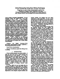
Spectral plots for sand beaches, gravel beaches, and manmade structures ....................43

B-1

Spectral plots for scrub-shrub and salt marshes in the four IKONOS bands ...............B-4

B-2

False color image bands 4,3,2.......................................................................................B-5

B-3

IKONOS Band 4 shown as 5 natural breaks.................................................................B-5

ix

B-4

NDVI of IKONOS imagery shown as 5 natural breaks................................................B-6

B-5

IKONOS tasseled cap band 2 (greenness) shown as 5 natural breaks..........................B-6

B-6

All four bands of the tasseled cap image ......................................................................B-7

B-7

The brightness and greenness bands of the tasseled cap image....................................B-8

B-8

Attributes of classified GVI ..........................................................................................B-9

B-9

Attributes of classified 4-band Image ...........................................................................B-9

x

LIST OF TABLES Table

Page

1

Acquisition details for the archived IKONOS imagery.......................................................3

2

Standard ESI shoreline types mapped during the field work to collect in situ data ............5

3

Modified shoreline classification.........................................................................................6

4

Summary of the classification accuracy assessment..........................................................10

C-1 Overall error matrix .........................................................................................................C-4 C-2 Seaward error matrix .......................................................................................................C-6 C-3 Landward error matrix .....................................................................................................C-6

xi

ABBREVIATIONS, ACRONYMS, AND SYMBOLS

cm CASI DGPS ESI GIS GVI G-WIS km LDWF LiDAR LSU LUMCON m mm MMS NDVI NOAA OCS RPI T-Cap

centimeter Compact airborne spectrographic Imager Differential global positioning system Environmental Sensitivity Index Geographic Information Systems Greenness Vegetation Index Gulf-Wide Information System kilometer Louisiana Department of Wildlife and Fisheries Light Detecting and Ranging Louisiana State University Louisiana Universities Marine Consortium meter millimeter Minerals Management Service Normalized Difference Vegetation Index National Oceanic and Atmospheric Administration Outer Continental Shelf Research Planning, Inc. Tasseled Cap Transformation

xiii

1.0

INTRODUCTION

Environmental Sensitivity Index (ESI) mapping refers to a shoreline classification and sensitivity ranking system that has been a vital component of oil spill contingency planning and marine environmental assessment programs nation wide for 25 years (Halls et al., 1997). The U.S. Minerals Management Service (MMS) currently uses ESI data and the ESI classification scheme for environmental assessment studies related to Outer Continental Shelf (OCS) activities. Traditional ESI data development includes the interpretation of aerial photographs and mapped observations by coastal geologists during overflights. This method has been applied successfully to the majority of the U.S. coastline. The complex, rapidly changing shoreline of Louisiana, however, has made ESI mapping extremely difficult using traditional techniques. As a result, a coast-wide ESI shoreline classification has never been developed for Louisiana. This represents a major information gap, as oil spill risk and environmental consequences in Louisiana are great. ESI classification efforts in Louisiana in the late 1980s relied on remotely sensed imagery with spatial resolution of 20-30 meters (Jensen et al., 1990). Although a useful landuse/land cover classification was achieved, the detail associated with the linear nature of shoreline features could not be resolved, and a true ESI shoreline classification was not possible. More recently, the barrier island beaches and other outer-coast features of Louisiana were classified using traditional ESI methods, as part of the Gulf-Wide Information System (G-WIS) project (MMS et al., 2001; Zengel and Hanifen, 2001; Zengel et al., 2002). This effort was possible due to the linear configuration of the outer coast. Beyond this, most of the Louisiana coast remains unclassified and cannot reasonably be completed using traditional methods. Newer, high-resolution satellite imagery offers the best opportunity for coast-wide ESI shoreline mapping and classification in Louisiana and other similar areas with highly complex, rapidly changing shorelines. The primary objective of this research was to develop remote sensing classification procedures to support ESI mapping efforts in Louisiana and elsewhere. Several questions comparing remote sensing techniques and traditional classification methods were of interest including: • Are remote sensing methods reliable, more cost and time effective, and do they provide as much information as traditional methods? • Is the spectral and spatial resolution of the IKONOS satellite imagery chosen for the project appropriate? • Is the use of archived imagery for cost savings appropriate? • Can a viable land/water interface be created from the imagery? • Can an ESI style product useful for spill response and coastal management be produced? The saline areas of the Louisiana coastline from Port Fourchon to Lake Barre were chosen as the study site (Figure 1). Salinity boundaries were obtained from the 1997 Louisiana Coastal Marsh Vegetative Type Map (LDWF et al., 1997), which included values of brackish, fresh, intermediate, saline, and water. In this data set saline was defined as salt marsh having typical vegetation of oystergrass (spartina alterniflora), glasswort (avicennia germinans), and saltgrass (distichlis spicata). This area of coastal Louisiana has experienced high rates of land loss and rapid shoreline change that have made traditional ESI classification techniques difficult. However, the presence of extensive oil and gas infrastructure and highly sensitive habitats and

1

natural resources in this area emphasizes the need for up-to-date maps for oil spill planning and response. 2.0

METHODS OF STUDY

2.1

Introduction The study methodology consisted of the following tasks: image acquisition, land/water interface production, in situ data collection, image classification, vector shoreline transfer, validation overflight, and an accuracy assessment. In contrast, a traditional ESI project methodology would consist of: identification of existing digital land/water or shoreline, overflight classification on topographic quads, field classification accuracy assessment, and onscreen ESI attributing of the digital shoreline.

Figure 1. Entire study area and image swaths. The swaths outlined in bold comprise the study area for the ESI classification (see Table 1 for image details). 2.2

Image Acquisition Archived IKONOS 4-band multispectral, 4-meter (m) spatial resolution imagery was selected for use in this study. It was hoped that the 4-meter pixel resolution of the IKONOS

2

satellite would capture narrow features such as sand beaches that are missed by 20 and 30-meter resolution products. It was also hoped that archived imagery would prove cost-effective for a large study area and could thus allow for more frequent ESI updates. Seventeen images were collected for the study area and used for the creation of the land/water interface; three were replaced and not used because of extensive cloud cover. These three images are not labeled in Figure 1. A subset of the saline areas of eight images was chosen for the ESI classification. These eight images were acquired during different dates, seasons, tidal cycles, winds, and different atmospheric conditions (Table 1). The effects of these variables are discussed throughout this report. Table 1 Acquisition Details for the Archived IKONOS Imagery

Tile Index A B C D E F G H I J K L M N

14 13 12 11 9 8 7 5 17 6 2 1 15 16

Acquisition Date

Acquisition Time (GMT)

1/7/2002 1/7/2002 12/27/2001 11/5/2001 3/11/2002 3/22/2002 3/22/2002 4/24/2002 9/25/2003 3/22/2002 1/7/2002 12/27/2001 9/25/2003 9/25/2003

16:53 16:53 16:52 16:56 16:49 16:50 16:50 16:52 17:03 16:50 16:53 16:52 17:03 17:02

2.3

Acquisition Time (Central Standard) am 10:53 10:53 10:52 10:56 10:49 10:50 10:50 10:52 11:03 10:50 10:53 10:52 11:03 11:02

Tide Mid Mid Low Low Low High High High

Generation of the Land/Water Interface For planning and logistics the land/water interface provides a useful tool for coastal management and oil spill response. In the production of an ESI atlas, the land/water interface is an important component that represents the shoreline on which the habitat classifications are attributed and assists in data summary and legibility of the cartographic product. Infrared light is strongly reflected by healthy vegetation and is highly absorbed by water, making it excellent for developing a land/water interface. The Landsat Thematic Mapper satellite has three infrared bands ranging from near to mid-infrared, and has been effectively used for developing water indices and models for land/water interface delineation. The mid-IR bands are particularly good for detection of wetness and water. The IKONOS satellite however, has but one infrared band in the near region, and consequently is less effective for water detection and land/water interface development. In addition, models developed using multiple IR bands for the Thematic Mapper cannot be directly applied to IKONOS.

3

The single IKONOS infrared band was initially level-sliced to derive a land/water threshold, but the result was not adequate. A normalized difference vegetative index (NDVI) was produced using the standard ratio of visible-red and infrared bands. The level-slice and threshold of the NDVI also proved inadequate for clearly separating land and water in the complex, low marsh environment of Louisiana. Therefore, we resorted to a proven but time-consuming method -- the ISODATA unsupervised classification algorithm was employed using the green, red, and infrared bands of the IKONOS imagery with 75 initial classes. The ISODATA signatures were inspected for homogeneity and normality, and then processed with the Maximum Likelihood Decision Rule to classify the image. Probabilities were assigned based on class counts. This was completed independently for each image since they were acquired on different dates and had different water levels. The individual spectral classes were categorized into land or water to create a thematic land/water binary image. Confused classes (transition classes showing both land and water) were masked and differentiated by running ISODATA on the subset of image pixels assigned to the class - separating them into discrete spectral categories that were further defined as land or water. Islands of land or water smaller than .5 acres were eliminated from the classified image. A recursive cross-majority filter was applied to smooth the land/water interface edges and to minimize acute spurs. The land/water classified raster images were converted to vector polygons using a rasterto-vector algorithm with a weed tolerance slightly smaller than the inherent cell size of the IKONOS imagery. The polygons were attributed with a grid code and class field, each polygon defining either a water body or land area. Finally, the polygon files were also topologically converted to lines representing the shore or land/water interface. Figure 2 shows the vectorized land/water interface displayed over a small portion of an original satellite image. Two IKONOS scenes had problems with clouds. Multi-temporal images with broken clouds were acquired of each scene. The clouds were removed using a replacement model when cloud free imagery was present from at least one image. Clouds that could not be removed were classified as clouds when it could not be determined what was below them. 2.4

In situ Data Collection During October 12-17, 2003, a team consisting of a coastal geologist and a remote sensing analyst visited 211 field sites to assist in the habitat imagery classification. Data collected included a GPS location, photos of the site, and a description of the morphology and vegetation. During the field work, the coastal geologist identified thirteen standard ESI classes (Table 2) that were present within the study area. Sites were chosen to cover all of the classes identified and were primarily visited by boat. 2.5

Classification Methodology A series of image analysis techniques were applied to the imagery to test whether the standard ESI classifications could be extracted from the IKONOS imagery. After a series of algorithms and methodologies were tested and applied it was concluded that the same level of classification detail in the standard ESI could not be extracted from the IKONOS imagery. Based on this assessment, the coastal geologist created the modified shoreline classification (Table 3) that was used in the methodology below to create the final classifications.

4

Figure 2. IKONOS satellite image overlaid with vectorized land/water interface derived from the image. Table 2 Standard ESI Shoreline Types Mapped during the Field Work to Collect In Situ Data ESI Shoreline Type 1B 2A 2B 3A 6A 6B 7 8A 8B 8C 9A 10A 10D

Definition Exposed solid man-made structures (e.g., seawall, bulkhead, etc.) Exposed wave-cut platforms in mud Exposed scarps or steep slopes in mud Fine to medium-grained sand beaches Shell beaches Exposed riprap Exposed tidal flats Sheltered scarps in mud Sheltered solid man-made structures (e.g., seawall, bulkhead, etc.) Sheltered riprap Sheltered tidal flats Salt- to brackish-water marshes (including intermediate marshes) Scrub-shrub wetlands (including mangroves)

5

Table 3 Modified Shoreline Classification Class Beaches and manmade structures

ESI Class 1B, 3A, 6A, 6B, 8B, 8C

Mud and tidal flats

2A, 2B, 8A, 9A, 7

Salt marsh

10A

Shrub-scrub

10D

Examples Seawalls, urban infrastructure, sand beaches, gravel beaches, riprap Wave cut scarps in mud, exposed tidal flats, sheltered tidal flats, oyster beds Spartina alterniflora, Spartina patens Mangroves, vegetated banks, scrub-shrub

The basic methodology for the modified shoreline classification is outlined in Figure 3. In Step 1, the image classification methodology was to clip the 4-band image to the saline area. In Step 2, an unsupervised ISODATA classification was run on the saline area of the image to separate the areas of land from areas of water. The ISODATA classification separated the pixels into spectrally similar groups. The pixels classified as land were masked out of the original 4band image, creating a new image with only the saline land areas. In Step 3, a Tasseled Cap Transformation (T-Cap) was run on the saline land image. The T-Cap is a vegetation index that is effective at distinguishing between vegetation and non-vegetation classes (Jensen, 1996; 2000; Horne, 2003). An unsupervised ISODATA classification was run on the T-Cap image to group the vegetation and nonvegetation classes. The areas of vegetation were masked out of the T-Cap image to create a vegetation image. The areas of nonvegetation were masked out of the original 4-band image to create a nonvegetation image. In Step 4, an unsupervised ISODATA classification was run on the nonvegetation image. Results from this classification were used to determine the beaches and manmade structures class and the mud and tidal flats class. In Step 5, an unsupervised ISODATA classification was run on the vegetation image. Results from this classification were used to determine the scrub-shrub class and the salt marsh class. The in situ data points, field notes, and photographs were used to assign habitat values to the spectrally similar classes in steps three, four and five. The final step in the classification methodology was to merge the individual classification images back into a single image. After the classification methodology was complete, a 3 by 3 smoothing algorithm was applied to the classification to reduce the amount of speckle. The smoothing algorithm was not applied to the beaches and manmade structures because these features are often narrow, short, and might be eliminated during smoothing. Refer to Appendix A and B for a detailed explanation of the classification procedures.

6

Figure 3. Image classification methodology. 2.6

Shoreline Transfer The imagery classification results are inherently area classifications that place all pixels in the image into one of the defined classes. In the traditional ESI approach, classifications are attributed directly to the linear shoreline feature. This approach provides summarized data in an easy to interpret format for the spill responder and aids in creating cartographic products (e.g., an image can be placed underneath the linear classification giving further locational information to the responder). To emulate the traditional product, the area/polygonal image classification was transferred to the linear land/water interface created previously in the project. The general methodology is presented in this section. First, the land/water interface was generalized to remove the "stair stepping" from the pixelated imagery. The generalization procedure removes line vertices within a specified tolerance to reduce the complexity of the shoreline. A tolerance of 5 meters was selected for the generalization, which produced a shoreline sufficient for viewing at the typical ESI scales between 1:10,000 and 1:24,000 (Figure 4). Next, sample points were generated at 10 m intervals along the shoreline. Area of influence or Thiessen polygons were then generated for each sample point, and the shoreline was buffered at a 5 m interval in the water and 5, 10, and 20 meter intervals on the land (Figure 5). These Thiessen buffers were then overlaid with the polygonal ESI classification and were characterized by the maximum area of ESI type in each buffer (Figure 6). The results were then collapsed to the shoreline based on a locational ID on the Thiessen polygons. Finally, the collapsed results were formatted to the same style as the traditional ESI product.

7

1:3,000 1:10,000

Figure 4. Generalization of the shoreline. The 1:3,000 frame shows the original land/water interface in black and the generalized shoreline in red. The 1:10,000 frame shows the same area at a smaller scale. The generalization removed the “stair step” effect by reducing shoreline detail. This reduction in detail is difficult to notice at the scales at which ESI maps are typically produced and used.

Figure 5. Shoreline sampling intervals and buffers used to attribute the shoreline with the habitat classification.

8

Figure 6. Habitat characterization for the sample intervals and buffers.

2.7

Validation Overflights Overflights were conducted during 6-8 February 2004 to test the accuracy of the shoreline habitat classification. These flights covered images A through H, exclusive of E, which had a large amount of cloud cover (Figure 1). The overflights were conducted within four hours of low tide. The Traditional ESI classification (Table 1) were mapped during the flights onto plots of the images that had the modified classes of sand beach/man-made structures, salt marsh, and scrub-shrub attributed to the shoreline and the modified class of mud plotted as polygons. Image A and part of Image B were mapped on 6 February as a front was starting to come through and the water levels in the study area reflected normal lunar tidal influences. Images B, C, and D were mapped on 7 February under strong north wind conditions that created a “wind tide” that was markedly lower than the normal lunar tide. Many more tidal flats and wave-cut platforms were mapped during these lower water levels. Images F, G, and H were mapped on 8 February, after the front had passed and the normal southeast wind pattern had returned, along with normal water levels. 2.8

Accuracy Assessment An error matrix based on the length of shoreline in each class was created to assess the accuracy of the image classification against the classification mapped during the overflights and is shown in Appendix C. The overall accuracy of the classification was 98.02%. This accuracy assessment indicates that the methodologies outlined in this research are effective at classifying broad ESI classes. However, it is important to note that this is an assessment of the generalized/modified ESI categories, which contributed significantly to the high accuracy rating.

9

The classification accuracy assessment is summarized (Table 4) as the percentage of over- and under-classified modified classes on both the seaward and landward sides of the shoreline. The over and under classification refers to the percentage of error that was either over classified (user’s accuracy and commission error) or under classified (producer’s accuracy and omission error). Commission error is over inclusion of a particular class. Omission error is exclusion of a particular class (Jensen, 1996). A brief explanation of the classification error is listed in Table 4. Refer to Appendix C for the detailed accuracy assessment. Table 4 Summary of the Classification Accuracy Assessment Modified Class Beaches and manmade structures

Classification Over

Seaward 26.63%

Landward 7.60%

Explanation Over classification was expected because this class was not filtered or smoothed Under 8.56% 16.48% Features smaller than 4 meters could not be classified using the IKONOS imagery.* Mud and tidal flats Over 1.55% 3.23% Wet sand and “coffee ground” type features over classified as mud and tidal flats. Under 1.20% 0.22% Under classification was expected from image tiles collected at higher tides. Scrub-shrub Over 16.38 % 14.47% Over classification is likely due to mixed classes of scrub-shrub and salt marsh. Small patches of salt marsh, other than the Spartina, such as fragmities, classified more like scrub-shrub than salt marsh. Under 2.07% 2.69% Areas of under classified scrub-shrub occurred in the northern reaches of the imagery. Differences in species type could lead to under classification. Salt marsh Over 0.52% 0.19% A relatively small length of salt marsh was over classified on either seaward or landward sides of the shoreline Under 1.63% 0.68% Small patches of salt marsh grow on the seaward side of other classification types. These small patches are too small to be classified from the IKONOS imagery. *Since the resolution of IKONOS multispectral imagery is 4 meters, it is not generally possible to develop spectral signatures for land cover classes smaller than the inherent resolution of the sensor. In fact, to develop statistically reliable signatures requires 25 or more pixels (samples). Individual isolated pixels are mixed with surrounding classes too much to reliably identify. These are usually misclassified.

3.0

RESULTS The results section describes ten ESI habitat types that were observed during the field work and traditional overflights. For each ESI habitat type, the habitat characteristics are described, and the technical performance of the imagery and classifications techniques are discussed. The text is followed by a subset of the IKONOS imagery where the ESI habitat is present, a second set of images shows the imagery with the shoreline classification. An oblique aerial photograph, taken during the overflights, is shown for the same general area of the imagery, and finally a representative ground photograph is provided for each ESI habitat.

10

EXPOSED WAVE-CUT PLATFORMS IN CLAY

ESI = 2A

Habitat Description • •

•

•

•

The intertidal zone is a flat, muddy platform or bench of variable width. The sediments may incorporate a high percentage of organic material and root masses from eroding salt marsh vegetation. Often the platform is covered by a thick accumulation of loose organic particles known as “coffee grounds.” They are regularly exposed to moderate to high wave energy from wind-generated waves where they occur along water bodies with significant fetch towards the south and southeast. They most commonly occur along the outer Gulf coast or the seaward headlands of marsh islands on the north side of the larger bays. There is always at least one other habitat present on the landward side, usually a sand beach, gravel (shell) beach, salt marsh, or scrub-shrub vegetation. Sometimes, there are two landward habitats present. Very occasionally there is an exposed tidal flat seaward of the platform. In the aerial photograph in figure ESI 2A, note that the wave-cut platforms occur along the most exposed front sides of the marsh islands. With a paucity of sediments, the landward side of the platform consists of eroding salt marsh and scrub-shrub.

Technical Performance of the Imagery Classification •

The ability to accurately classify exposed wave-cut platforms in clay from IKONOS imagery is dependent on the tidal stage at which the imagery is acquired. The importance of tidal range is evident when comparing IKONOS imagery acquired at high vs. low tides and in comparison to aerial overflights at low tide (see appendices for details). The imagery shown in figure ESI 2A (A & B) was acquired at a higher tide than the validation overflights, which were conducted during a north wind event that created an even lower “wind tide.”

•

Based on the results from other image tiles acquired at low tides, it is reasonable to conclude that had this image been acquired at a lower tide, the tidal flats would have been accurately classified.

•

Recommendation: acquire imagery at the lowest tide possible.

Figure 7(a-d) illustrates ESI 2A, Exposed wave-cut platforms in clay.

11

Figure 7-a. False-color IKONOS imagery acquired April 24, 2002 (Figure 1, Tile H).

Figure 7-b. The imagery classification was both mud and scrub-shrub. Where the platform was wide, it could be identified using the 4 meter imagery, but narrow platforms were classified as the landward vegetation.

12

Figure 7-c. Aerial photograph of the area in figure A, but looking to the west, taken on 8 February 2004.

Figure 7-d. Ground photograph (October 2003) of the area just west of the Port Fourchon jetties. Here sand beaches are eroding, exposing the salt marsh peat sediments and young mangrove vegetation. Also refer to figure ESI = 3A for the aerial photograph and imagery for this location.

13

EXPOSED SCARPS AND STEEP SLOPES IN CLAY

ESI = 2B

Habitat Description •

Intertidal zone is a vertical scarp that is generally more than 1-1.5 m high and composed of muddy, consolidated sediments.

•

The sediments may incorporate a high percentage of organic material and root masses from eroding marsh vegetation.

•

They are regularly exposed to moderate to high wave energy, either from wind-generated waves where they occur along waterbodies with significant fetch towards the southeast or north, or from boat wakes in high-traffic corridors.

•

They are usually backed by scrub-shrub vegetation, although salt marshes and gravel (shell) beaches can also occur landward of the scarp. There is no shoreline type seaward of the scarp.

•

They are only mapped as a separate habitat type when the scarp is at least 1 m high.

•

They are uncommon along the coast of Louisiana. Along the most exposed shorelines, the waves cut a flat bench or platform rather than a vertical scarp, so the scarps tend to occur on the edges of marsh islands, along inner waterbodies, and along high-traffic canals.

•

In Figure ESI 2B, the tip of the small island was mapped as a double shoreline, with scrub-shrub fronted by exposed scarps and steep slopes in clay (10D/2B).

Technical Performance of the Imagery Classification •

The IKONOS imagery could not extract vertical features, such as ESI class 2B. Rather, exposed scarps are classified as the habitat type on top of the scarp.

•

In instances where the scarp is sloping and/or not covered by vegetation, that area could conceivably be classified.

•

This ESI class is less dependent on the tidal stage for accurate mapping.

•

Recommendations: To accurately classify ESI 2B, a methodology that can extract vertical features is necessary. It is possible that the addition/use of ancillary elevation data or imagery that contains a vertical component could improve the classification. With the advent of LIDAR derived elevations for coastal Louisiana, this is highly possible.

Figure 8(a-d) illustrates ESI 2B, Exposed scarps and steep slopes in clay.

14

Figure 8-a. False-color IKONOS imagery, obtained on March 22, 2002 (Figure 1, Tile F).

Figure 8-b. The imagery classification was scrub-shrub. Because of the narrow, vertical scarp, this habitat type cannot be identified using the 4 m imagery.

15

Figure 8-c. Aerial photograph taken on 8 February 2004. The arrow points to the small island that was mapped during the overflights as both shrub-shrub and exposed scarps (10D/2B).

Figure 8-d. Ground photograph of an exposed scarp along a waterway (October 2003). The scarp is generally vertical, composed of consolidated, muddy sediments. Note the eroding blocks of mud at the base of the scarp and the exposed roots of live vegetation, indicating active erosion. No habitat type occurs seaward of the scarp. Scrub-shrub habitat usually occurs on the landward side of the scarp.

16

FINE- TO MEDIUM-GRAINED SAND BEACHES Habitat Description

ESI = 3A

•

Intertidal zone is composed of a wide, flat, and hard-packed sand beach.

•

The sediments are very mature, consisting mostly of quartz grains and shell fragments.

•

They are exposed to moderate to high wave energy.

•

They are usually backed by low dune vegetation because, in most places, they are actively eroding across an older marsh surface.

•

In areas of high erosion, they are fronted by a wave-cut platform in clay (ESI = 2A).

•

They are common along the outer coast of Louisiana near sources of sand sediments, such as on barrier island or downdrift of headlands created by active or relict distributaries.

Technical Performance of the Imagery Classification •

Dry sand beaches exhibit spectrally bright values similar to manmade structures (asphalt and concrete) and clouds. IKONOS imagery is able to distinguish between spectrally bright features from all other feature types. However, the 4-band multispectral resolution of the IKONOS imagery is not high enough to distinguish between geographic features of similar spectral qualities, such as sand, manmade structures, and clouds (see section 4.0 for details).

•

Narrow beaches were not picked up by the imagery and classified as the surrounding habitats.

•

Submerged or damp sand were sometimes classified as mud and tidal flat.

•

Recommendations: More robust sensors, such as hyperspectral and/or airborne sensors, may be able to distinguish between different substrate types such as course sand, mud, and gravel beaches and manmade features.

Figure 9(a-d) illustrates ESI 3A, Fine- to medium-grained sand beaches.

17

Figure 9-a. False-color IKONOS imagery, acquired on January 7, 2002 (Figure 1, Tile A).

Figure 9-b. The imagery classification was sand beaches and man-made structures. Sand beaches appear very bright and are readily mapped using the imagery. This area was mostly classified as beaches and manmade structures. The jetty to the right was not classified and some areas of damp sand were classified as mud and tidal flat.

18

Figure 9-c. Aerial photograph taken on 6 February 2004. The beach occurs as a thin layer of sand that is being washed onto the old marsh surface as the shoreline erodes.

Figure 9-d. Ground photograph of the beach west of Port Fourchon (October 2003). This area was mapped as a double shoreline, with a fine-grained sand beach fronted by a wave-cut platform in clay (3A/2A). The width of both features makes them readily mapped using the IKONOS imagery.

19

GRAVEL (SHELL) BEACHES

ESI = 6A

Habitat Description •

Gravel beaches are composed of sediments larger than 2 mm that are mostly made up of shell (oyster) fragments in Louisiana.

•

The slope of the intertidal zone is intermediate to steep, compared to sand beaches.

•

Along the outer coast, they occur as multiple, wave-built berms and washovers usually forming the upper beach. Washovers are mounds of shells deposited by storm waves on top of the land surface above the normal high tide.

•

Along inner water bodies they are common as perched berms and washovers on scarps along high-traffic channels and canals where boat wakes provide the wave energy.

Technical Performance of the Imagery Classification •

Gravel Beaches reflect brightness values that are similar to sand and shell beaches and riprap and other man-made structures. The spectral signature of these ESI types can be identical, making distinguishing between the features unfeasible with the 4-band, 4-meter IKONOS imagery (see section 4.0 for details.)

•

Comparing the unclassified image (Figure A) with the classified image (Figure B), the long beach was classified correctly. However, the patches of beach to the right of the long beach, did not classify as accurately.

•

Recommendations: More robust sensors, such as hyperspectral and/or airborne sensors, may be able to distinguish between different substrate types such as course sand, mud, and gravel beaches. A sensor with a higher spatial resolution may be able to pick up the smaller beaches that were missed by the IKONOS imagery.

Figure 10(a-d) illustrates ESI 6A, Gravel (shell) beaches.

20

Figure 10-a. False color IKONOS imagery, acquired on January 7, 2002 (Figure 1, Tile A).

Figure 10-b. The imagery classification was beaches and man-made structures. The long beach correctly classified as a beach or manmade structure.

21

Figure 10-c. Aerial photograph taken on 6 February 2004 of a gravel (shell) beach along Bayou Lafourche. The bright white oyster shells occur as washover berm on the marsh surface created by large boat wakes along waterways with heavy traffic by large vessels.

Figure 10-d. Ground photograph (October 2003) showing the steep nature of the intertidal zone typical of gravel beaches.

22

RIPRAP

ESI = 6B

Habitat Description •

Riprap consists of man-made structures composed of cobble- to boulder-sized rock fragments or other miscellaneous debris.

•

They are called revetments when used onshore for shoreline protection, groins when used to trap sediments, jetties when used for inlet stabilization, breakwaters when used offshore, and canal plugs when used to close off pipeline and other types of canals (Figure C).

•

Riprap forms a steep slope (Figure D), the structures are usually large (several meters wide) to be effective.

•

Riprap is relatively common in developed areas, particularly along the larger navigational channels and associated with industrial sites (e.g., ports and oil facilities)

Technical Performance of the Imagery Classification •

The classification procedures were able to accurately classify these features shown in images below, as noted by the double-ended arrow. The single arrow is pointing to a thin, linear riprap feature, similar to that shown in the ground photo, but not shown in the unclassified imagery. Thus, the classification procedures inaccurately mapped a linear beach and man-made structure that does not appear in the unclassified imagery.

•

The narrow width of the features, algal growth on such features, and the vertical characteristic are possible reasons for the misclassification of these features.

•

Recommendation: A sensor with higher spatial and spectral properties may improve the classification results of riprap (refer to Section 4.0 for details).

Figure 11(a-d) illustrates ESI 6B, Riprap.

23

Figure 11-a. False color IKONOS Imagery, acquired on January 7, 2002 (Figure 1, Tile A).

Figure 11-b. The imagery classification was beaches and man-made structures. The section of riprap in this figure was correctly classified as beaches or man-made structures, denoted by the double arrow.

24

Figure 11-c. Aerial photograph taken on 7 February 2004 of riprap used to plug the pipeline canals. Note the gravel beach to the east (right) of the structure, and that it was not possible to differentiate between the riprap and gravel using the IKONOS imagery classification.

Figure 11-d. Ground photograph of riprap along Bayou Lafourche, a heavily trafficked waterway (October 2003). Note the steepness of the intertidal zone and the typical width of the structure.

25

EXPOSED TIDAL FLATS Habitat Description

ESI =7

•

These are flat, unvegetated intertidal areas, composed primarily of sand with some mud and shell, that vary in width from a few to hundreds of meters.

•

The presence of sand indicates that tidal or wind-driven currents and waves are strong enough to mobilize the sediments. Therefore, they are located mostly along the outer coast where they are exposed to waves (Figure C).

•

They are usually associated with another shoreline type on the landward side of the flat.

•

Exposed tidal flats are widest where they are associated with sand beaches, such near Port Fourchon (Figure D).

Technical Performance of the Imagery Classification •

The largest influence on the mapping of flats was the tidal stage at which the imagery was acquired.

•

This imagery was acquired during a tidal cycle low enough to accurately classifying the tidal flats.

•

Recommendations: When the imagery is acquired during lower tides, the classification process is effective at accurately classifying tidal flats. For consistent mapping between imagery tiles, it is important to collect imagery within the same tidal range.

Figure 12(a-d) illustrates ESI 7, Exposed tidal flats.

26

Figure 12-a. False Color IKONOS imagery, acquired on November 5, 2001(Figure 1, Tile D).

Figure 12-b. The imagery classification was mud and tidal flats. The classification correctly mapped the extensive flats in this figure.

27

Figure 12-c. Aerial photograph of exposed tidal flats along a marsh island on the outer coast, taken on 7 February 2004. The view is looking northeast. Exposed tidal flats are widest on either side of the small peninsula.

Figure 12-d. Ground photograph of the wide sandy tidal flat near the jetties at Port Fourchon (October 2003). Such wide flats are associated with barrier islands and headlands.

28

SHELTERED MAN-MADE STRUCTURES Habitat Description

ESI = 8B

•

Sheltered man-made structures include revetments, seawalls, piers, and docks typically constructed of impermeable materials such as concrete and wood.

•

They occur inside harbors and in front of developed properties (camps and oil facilities) along canals and waterways.

•

They are usually vertical structures and do not occur with other shoreline types.

Technical Performance of the Imagery Classification •

Seawalls such as those shown in the overflight and field photos are not easily distinguishable in IKONOS imagery. The widths of seawalls are too narrow to be identified using 4 m spatial resolutions.

•

The classification procedures were unable to accurately detect these features.

•

Recommendation: A sensor with higher a spatial resolution may enable these linear seawalls to be classified correctly.

Figure 13(a-d) illustrates ESI 8B, Sheltered man-made structures.

29

Figure 13-a. False Color IKONOS imagery, acquired on January 7, 2002 (Figure 1, Tile B).

Figure 13-b. The imagery classification was beaches and man-made structures. The classification procedures did not accurately classify the seawalls. The seawalls were classified as the neighboring habitats.

30

Figure 13-c. Aerial photograph taken on 6 February 2004, with a view that is very similar to B. Vertical seawalls and docks have been built in front of the houses. There is water on the seaward side and developed land on the landward side.

Figure 13-d. Ground photograph (October 2003) of a seawall that is part of a structure to plug a pipeline canal. In this case, there is salt marsh behind the seawall. Seawall and riprap often intermixed along developed areas

31

SHELTERED TIDAL FLATS Habitat Description

ESI = 9A

•

Sheltered tidal flats are composed primarily of mud with minor amounts of sand and shell.

•

They are present in calm-water habitats, sheltered from waves and strong tidal currents. They occur along channels in salt marshes and as open, unvegetated areas within salt marsh habitat.

•

They can have heavy wrack deposits along the upper fringe.

•

The intertidal exposure of the tidal flat is strongly dependent on water level, which is affected by both astronomical and wind-generated tides. During strong north wind events, water is driven out of the shallow bays, exposing wide tidal flats. During normal southeast winds, most of the flats are covered by water.

Technical Performance of the Imagery Classification •

The classification of shallow water tidal flats is dependent on the tidal stage during which the imagery was acquired.

•

The sheltered (9A) and exposed (7) tidal flats classified the same. An exposure index applied to the classified image and/or shoreline can refine this broad mud and tidal flat class into exposed or sheltered tidal flats.

•

Oyster beds embedded in the mud and tidal flats can exhibit brighter spectral properties and lead to mud and tidal flats classified as beaches and man-made structures.

•

Recommendation: When feasible, acquire the imagery during the low tides. Use an exposure index to further define the tidal classes.

Figure 14(a-d) illustrates ESI 9A, Sheltered tidal flats.

32

Figure 14-a. False color IKONOS imagery, acquired on January 7, 2002 (Figure 1, Tile B), at low tide.

Figure 14-b. The imagery classification was mud and tidal flats. The classification procedures successfully classified the muddy tidal flats on this low-tide imagery.

33

Figure 14-c. Aerial photograph taken on 7 February 2004 during low tide and a strong north wind weather condition. Note that extensive areas of sheltered tidal flats are exposed. For orientation, note the canal in the right center of both the imagery and oblique aerial photograph.

Figure 14-d. Ground photograph (october 2003) of a sheltered tidal flat fringing salt marsh. The sediments are generally dark and organic rich. There can contain scattered patches of oysters.

34

SALT MARSHES Habitat Description

ESI = 10A

•

These are intertidal wetlands consisting of emergent, herbaceous vegetation that is salt tolerant.

•

Marshes vary in distribution from extensive areas of dense vegetation to broken marsh to fringing marshes.

•

Near the coast, small mangroves occur along the marsh fringe, where mangrove seedlings have stranded and taken root. Mangroves are generally killed every few years when a big frost occurs.

•

Marsh soils range from fine sands to mud, to organic-rich peats.

Technical Performance of the Imagery Classification •

Overall, the classification of salt marsh was effective, except in the highly broken up areas of marsh. The imagery below shows areas of broken marsh that were misclassified as mud and tidal flats.

•

Vegetation indices were used to classify the vegetated areas. The Greenness Vegetation Index, band 2 from the Tasseled Cap transformation, successfully distinguished salt marsh habitat from scrub-shrub habitat.

•

The salt marsh habitat is the dominant habitat throughout the study area.

•

Areas of exposed salt marsh and/or areas where the edge of the salt marsh had been flattened were more difficult to classify than the other areas of salt marsh habitat.

•

Recommendations: Acquire imagery at the height of the phenological cycle for the dominant vegetation. Apply additional algorithms to areas of broken marsh to improve the classification.

Figure 15(a-d) illustrates ESI 10A, Salt marshes.

35

Figure 15-a. False Color IKONOS Imagery, acquired on January 7, 2002 (Figure 1, Tile A).

Figure 15-b. The imagery classification was salt marsh. The classification of salt marsh in this area was successful. Some of the areas of broken marsh were misclassified as mud and tidal flats.

36

Figure 15-c. Aerial photograph taken on 7 February 2004 showing areas of extensive and broken marsh. For orientation, the small pond with a narrow channel on the east (lower) side of the channel in the middle of the imagery is also visible in the middle of the photograph, though the view is much more oblique.

Figure 15-d. Ground photograph (October 2003) of salt marsh habitat.

37

SCRUB-SHRUB WETLANDS Habitat Description

ESI = 10D

•

Scrub-shrub wetlands consist of salt-tolerant woody shrubs that grow 1-3 meters high.

•

Their lower limit is above the high-tide line because they do not tolerate regular saltwater inundation.

•

The width of the vegetation can range from one tree to a many kilometers.

•

They are common along canals on the side where the spoil was broadcast because the land elevation is higher.

Technical Performance of the Imagery Classification •

Overall, scrub-shrub vegetation was relatively easy to extract from the IKONOS imagery, however some images produced better results than others. The spectral signatures of vegetation are distinctly different from non-vegetation types. Within the study area in Louisiana, the main vegetation present was shrub-scrub and salt marsh. These two vegetation types have similarly shaped spectral profiles, with the main distinguishing factor being the near-infrared band (band 4). Refer to Appendix B for details.

•

Recommendations: Identify the vegetation cycles of the dominant vegetation types (saltmarsh and shrub-scrub) and acquire imagery when the vegetation cycles are the most different. Use additional image processing techniques, such as texture or height analysis to distinguish between salt marsh and scrub-shrub. Further analysis may be able to distinguish between mangroves and other types of scrub-shrub. Elevation data may be useful at distinguishing between scrub-shrub wetlands and vegetated banks. The classification could also be improved by using additional infrared spectral bands, applying a different classification algorithm, or by using all the T-Cap bands in the classification.

Figure 16(a-d) illustrates ESI 10D, Scrub-shrub wetlands.

38

Figure 16-a. False color IKONOS image, acquired on January 7, 2002 (Figure 1, Tile A).

Figure 16-b. The imagery classification was scrub-shrub. Scrub-shrub areas are easily identified in the imagery and appear and brighter reds at higher elevations.

39

Figure 16-c. Aerial photograph taken on 6 February 2004. The riprap canal plug in the distance in the photograph is visible as a bright line in the middle of the imagery. Scrub-shrub wetlands were readily differentiated from other wetland types, as can be seen by comparing the classified imagery and the aerial photograph.

Figure 16-d. Ground photograph (October 2003) showing the slightly supratidal elevation of the scrub-shrub vegetation and the typical mix of some salt marsh on the seaward side.

40

4.0 SUMMARY AND RECOMMENDATIONS FOR ADDITIONAL RESEARCH The spatial and spectral resolutions of IKONOS imagery adequately captured four broad habitat classes, but did not extract the same level of detail as traditional ESI mapping methods. The usefulness and applicability of these broad ESI classifications are dependent on the question at hand. For oil spill response, the relatively current imagery provides a valuable base map that is greatly improved over other available maps. This feature is particularly important in coastal areas experiencing rapid shoreline change. One of the biggest challenges of responders in these areas is access to maps that accurately reflect current conditions and shoreline locations so that equipment and personnel can be deployed to appropriate cleanup sites. Currently, responders obtain oblique digital photography during overflights, then print out the photographs to use as base maps for deploying equipment and mapping the distribution of oil. Recent imagery would provide a more uniform base map. Creation of an actual shoreline would also be of value to spill responders, since miles of shoreline oiled is a common metric used to measure the spill impact on linear shoreline types and track cleanup progress. Both archived and new-collect imagery were used in this study. The average price for archived imagery was $6.85 per km² whereas the average price for new-collect imagery was $12.89 per km². The archived imagery is significantly cheaper, however, the seasons and tides cannot be chosen and fieldwork cannot coincide with the collection of the imagery. On the other hand, it is still difficult to predict and plan for new-collect satellite imagery to coincide with the desired seasons, tides and cloud free days, and the small swath width of the IKONOS satellite cannot collect imagery for a large area in a single pass. General recommendations to improve the classification of all ESI habitat types include the use of more robust sensors, sensors that can extract vertical structures, ancillary elevation data, texture analysis, and an exposure index. The Compact Airborne Spectrographic Imager (CASI and CASI 2) and Light Detecting and Ranging (LiDAR) are robust airborne sensors that have the potential to extract ESI classes with greater detail. Larsen and Erickson (1998) used the CASI sensor to distinguish between substrate types such as course sand, mud, and gravel beaches and man-made features. LiDAR collects elevation data, which may be useful in classifying vertical structures. Applying an exposure index to the shoreline can further define the modified classes into sheltered and exposed. 4.1

Mud and Tidal Flats The tide at which the imagery was acquired significantly affected the accuracy of the mud and tidal flat mapping. IKONOS imagery accurately classified mud and tidal flats when the imagery was acquired at low tide. When the imagery was acquired at high tides, few flats were classified. The validation overflights, conducted during low tide, confirmed the extensive areas of mud and tidal flats found within the coastal region of Louisiana. As identified in this research, imagery acquired at the lowest tide possible will improve the classification of mud and tidal flats. When using archived imagery, there is less option for choosing the tide. Commissioning imagery at specific dates and/or time, or collecting archived imagery based on tidal stage predictions would be difficult to implement. Within the study area, a north-south tidal gradient of ebb and flow was evident in the imagery. Thus, acquiring imagery where the entire image is at low tide may not be possible. One of the objectives of this study was to determine the feasibility of using archived imagery since it is cheaper. The limited selection available with regard to tidal conditions is

41

obviously a drawback. It would be better to use recently collected or commissioned imagery to target low tides, however, this is more expensive. There will be more options available in the near future as more high-resolution satellites are being developed and digital photography is becoming a competitive alternative. These platforms will provide pricing competition, better selection, improved capability, and more opportunity to acquire imagery at desired conditions. Future missions should consider these possibilities. 4.2

Beaches and Manmade Structures The modified ESI class of beaches and man-made structures was the most difficult and least accurate classification type. The spatial and spectral resolutions of IKONOS imagery are not as effective at distinguishing between spectrally bright features and/or narrow or vertical structures. Gravel and sand beaches, urban infrastructures, riprap, and seawalls all exhibit similar reflectance values within the multi-spectral IKONOS imagery. Figure 7 shows the overlapping spectral curves of known sand beaches, gravel beaches, and solid man-made structures in Tile A of the study area (Figure1). These overlapping spectral values are one reason these ESI classes could not be distinguished from each other. Another problem with classifying this habitat type was the suspended sediment in shallow water. Suspended sediment in shallow water has a higher radiant flux back to the atmosphere than nonturbid, clear water. Water with high concentrations of plankton and/or other organic matter also has a higher radiant flux than nonturbid water (Jensen, 2000). This higher radiant flux can lead to misclassification of the shallow water and/or turbulent water as a mud or tidal flat or beaches and man-made structures. In addition, the glare that reflects off the top of mud and tidal flats appears bright and is misclassified as beaches and man-made structures. The 4 m spatial resolution was not precise enough to consistently distinguish the linear characteristics of small beaches, riprap and other manmade structures. Some areas of riprap, usually multiple pixels in length and width, were classified as the modified ESI class of beaches and manmade structures while many areas of small beaches and/or manmade structures were not classified at all. Because these small habitats were not detected, they were classified as the dominant class surrounding them. Because the spectral properties alone cannot distinguish between the beaches and manmade structures, other methods should be tested to improve the classification of beaches and manmade sturctures: • Higher spectral and spatial resolutions • Texture analysis • Ancillary data Orun (2004) applied a texture analysis to distinguish between manmade and natural features using 5 m imagery. Initial investigation indicates that a texture analysis would increase the ability to distinguish between beaches and manmade structures, and potentially could distinguish between sand beaches and gravel beaches. Research into this approach may result in a methodology to distinguish between gravel beaches, sand beaches, and manmade features. A geometry analysis to distinguish between beaches and manmade features was unsuccessful because many small, linear beaches had similar dimensions as riprap and seawalls.

42

Figure 17. Spectral plots for sand beaches, gravel beaches, and manmade structures.

4.3

Scrub-Shrub Overall, the habitat class of scrub-shrub was easily identified and classified from the IKONOS imagery. Recommendations to refine the classification include: • Identifying the vegetation cycles of the dominant vegetation types (salt marsh and shrub-scrub) • Acquire imagery when the vegetation cycles are the most different • Applying a texture algorithm or elevation data may assist in further distinguishing between salt marsh and vegetated banks, mangroves and other scrub-shrub. 4.4

Salt Marshes Salt marsh was the dominant habitat class found within the study area. Overall, the classification of salt marsh habitats was successful. Research into the phenological cycles of scrub-shrub and salt marshes in Louisiana may be able to identify the month in which the phenological cycles are the most different. The classification of areas of broken marsh was less accurate than areas of solid salt marsh. Adapting a new methodology for areas of broken marsh may improve the classification results, particularly using all T-Cap bands or using more spectral bands. In addition, broken marsh areas could be defined by patch analysis.

43

5.0

REFERENCES CITED

Halls, J., J. Michel, S. Zengel, J.A. Dahlin and J. Petersen. 1997. Environmental sensitivity index guidelines, version 2.0. NOAA Technical Memorandum NOS ORCA 115, Seattle, Washington. 79 pp. plus appendices. Horne, J.H. 2003. A tasseled cap transformation for IKONOS images. In: ASPRS 2003 Annual Conference Proceedings in Anchorage, Alaska. Jensen, J.R., E.W. Ramsey, J.M. Holmes, J. Michel, B. Savitsky, and B.A. Davis. 1990. Environmental sensitivity index (ESI) mapping for oil spills using remote sensing and geographic information system technology. International Journal of Geographic Information Systems 4(2):181-201. Jensen, J.R. 1996. Introductory digital image processing: A remote sensing perspective. Prentice Hall, Upper Saddle River, New Jersey. Jensen, J.R. 2000. Remote sensing of the environment: An earth resource perspective. Prentice Hall, Upper Saddle River, New Jersey. Larsen, P.F. and C.B. Erickson. 1998. Applications of remote sensing and geographical information systems for marine resources management in Penobscot Bay, Maine: Intertidal habitat definition and mapping in Penobscot Bay. Report submitted to Island Institute by Bigelow Laboratory for Ocean Sciences. Louisiana Department of Wildlife and Fisheries (LDWF), Fur and Refuge Division; U.S. Geological Survey, Biological Resources Division's National Wetlands Research Center; and Department of Geography and Anthropology, Louisiana State University. 1997. 1997 Louisiana coastal marsh vegetative type map, geographic NAD83, LDWF, NWRC, LSU (1997) [salinity]: Louisiana Department of Wildlife and Fisheries, Fur and Refuge Division, and the U.S. Geological Survey's National Wetlands Research Center, Lafayette, Louisiana. Minerals Management Service, Louisiana State University, Louisiana Department of Wildlife and Fisheries, and Research Planning Inc. 2001. Gulf-wide information system, Louisiana: Outer coast environmental sensitivity index (ESI). U.S. Department of the Interior, Minerals Management Service, New Orleans, Louisiana. Arc/Info coverage and metadata. Orun, A.B. 2004. Automated identification of manmade textural features on satellite imagery by Bayesian Networks. Photogrammetric Engineering & Remote Sensing. 70 (2):211-216. Zengel, S. and J. Hanifen. 2001. Louisiana G-WIS: ESI, wildlife, and fisheries components. 17th Annual Louisiana Remote Sensing and GIS Conference, Baton Rouge, Louisiana, April 2-4, 2001.

44

Zengel, S., Z. Nixon, C. Plank, J. Hanifen, D. Sa, and D. Braud. 2002. Environmental sensitivity mapping and GIS: The Louisiana G-WIS database. Fourth Biennial Freshwater Spills Symposium in Cleveland, Ohio, March 19-21, 2002.

45

APPENDIX A Classification Methodology

A-1

General Polygonal Classification methods of IKONOS imagery: 1. Determine Study Area: a. Clip out original imagery to the upper salinity boundary. All imagery from here on out is clipped to this salinity boundary. 2. Determine Land vs. Water: a. Run an unsupervised classification (3-10 cl; depended on the image) on the original image to classify the water vs. land areas. b. Once the water/land distinction is made, mask out the water and land areas to create three images: - Mask of original image of water area only. - Mask of original image of land area only. - Classified image of water area with one class: water. 3. Using the land area mask of the original image, determine a vegetation class vs. a nonvegetation class. a. Run tasseled cap on the land area masked of the original image. b. Subset out band 2 (greenness) from the 4-band tasseled cap image. c. Run unsupervised classification (20-50 depending on the image) on band 2 (greenness) band of the tasseled cap image to determine a vegetation class from a nonvegetation class. d. Mask out the vegetation and nonvegetation classes from the unsupervised image. e. This step results in the following images: - 4-band tasseled cap image of the masked out land area of the original image. - Subset of band 2 (greenness) from the tasseled cap image. - Unsupervised classification of the Subset of band 2 (greenness) from the tasseled cap image. - Mask of vegetation class from the classified image. - Mask of nonvegetation class from the classified image. 4. Classify the nonvegation areas: a. Mask out the nonvegetation areas from the original 4-band image that was clipped to the saline boundary. b. Run an unsupervised classification (usually 20 class) on the 4-band image of the nonvegetation areas to determine the beaches and manmade structures class and the mud and tidal flats class. c. Use the field collected GPS points to assign class names to the unsupervised classification. d. Once the class names have been assigned, mask out the beaches and manmade structures class and the mud and tidal flats class. e. This step results in the following images: - Mask of the nonvegetation area from the original 4-band clipped image. - Classified image of the nonvegetation areas.

A-3

-

Mask of Classified image of the beaches and manmade structures Mask of Classified image of the mud and tidal flats

5. Classify the vegetation areas: a. Mask out the vegetation areas from band 2 (greenness) of the tasseled cap image. b. Run an unsupervised classification (usually 20cl) on band2 of the tasseled cap image mask of the vegetation areas to determine salt marsh from shrub-scrub. c. Use the field collected GPS points to assign class names to the unsupervised classification. d. Once the class names have been assigned, mask out the salt marsh and shrubscrub classes. e. This step resulted in the following images: - Mask of the vegetation areas from the band 2 of the tasseled cap image. - Classified image of the vegetation areas. - Mask of classified image of the salt marshes - Mask of classified image of the shrub-scrub. 6. Overlay the individual classification layers (water, beaches and manmade structures, mud and tidal flats, salt marsh, and shrub-scrub) into one classification image. 7. Use the 3 by 3 neighborhood function in ERDAS to ‘smooth’ out the speckeled nature of the classified image, excluding the beaches and manmade structures class from the smoothing algorithm. The beaches and manmade structures class is not smoothed because these features are often small and/or narrow and this smoothing could result in the loss of these important features. 8. Subset out the smoothed mud and tidal flats class. Convert the mud and tidal flats image into a polygon. This is the flats polygonal coverage.

A-4

APPENDIX B Detailed Classification Methodology for Vegetation Classes

B- 1

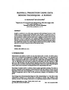
Initial unsupervised classification results were inconsistent in the classification of salt marsh and scrub-shrub habitat types. Fig. B-1 illustrates the overlapping spectral values of salt marsh and scrub-shrub that exist within the red and near infrared band. Healthy, green vegetation typically exhibits a strong spectral signal in the red and near-infrared bands. The relationship between the red and near-infrared band led to the development of remote sensing vegetation indices (Jensen, 2000). Vegetation indices are a dimensionless, radiometric measure of green vegetation that has been successful at classifying vegetation (Jensen, 1996; 2000). Numerous vegetation indices exist, including the Normalized Difference Vegetation Index (NDVI) and the Tasseled Cap transformation. Both the NDVI and Tasseled Cap were used on the IKONOS imagery to identify a methodology that would more accurately classify salt marsh and scrubshrub habitats. As shown in Fig. B-1, the main distinguishing factor between the scrub-shrub and salt marsh is the spectral reflectance in the near-IR band. The spectral values for each of the other three bands have relatively similar spectral profiles. Checking the imagery locations where a field verified scrub-shrub was classified as a salt marsh, the spectral reflectance for band 4 in those locations was closer to the spectral value of the salt marsh than the scrub-shrub. This event occurred relatively infrequently. Figure B-2 indicates areas of scrub-shrub and salt marsh. The scrub-shrub frequently occurs along the edge of the canal and the salt marsh predominately occurs in the inner area of the marsh and along the edge of the tidal creeks. Figure B-3 shows the near-infrared band with five statistical breaks, with the darkest colors mostly scrub-shrub areas. The NDVI created for the image, Fig. B-4, did not assist in the classification of the vegetation types. Kauth and Thomas developed the Tasseled Cap transformation for Landsat MMS imagery (Jensen, 2000). Horne (2003) derived a Tasseled Cap transformation specifically for use with IKONOS multi-spectral imagery. The Tasseled Cap Transformation results in four indexes, soil brightness index (SBI), green vegetation index (GVI), yellow stuff (YVI), and nonesuch index (NSI), which provide information about the separation between classes (Jensen, 1996; Horne, 2003).

B- 3

Figure B-1. Spectral plots for scrub-shrub and salt marshes in the four IKONOS bands.

The four equations derived by Horne (2003) are:

SBI = µ1= 0.326 xblue + 0.509 xgreen + 0.560 xred + 0.567 xnir GVI= µ2= -0.311 xblue – 0.356xgreen – 0.325xred – 0.819 xnir YVI = µ3 = -0.612 xblue – 0.312 xgreen + 0.722 xred – 0.081 xnir NSI = µ4= -0.650 xblue + 0.719 xgreen –0.243 xred – 0.031 xnir. Tasseled Cap transformation is useful at distinguishing between surface types (Jensen, 1996; Horne, 2003). This and other vegetation indices provide additional information about a scene that classification procedures cannot extract. The GVI was classified to identify the vegetation classes of salt marsh and scrub-shrub. The GVI is particularly useful in distinguishing between vegetation classes. The GVI from the Tasseled Cap transformation, Fig. B-5, did the best job at distinguishing between the scrub-shrub and salt marsh vegetation. Based on the results from the unsupervised classification, NDVI and Tasseled Cap transformation, the GVI was the chosen approach to classifying the vegetation classes.

B- 4

Scrub-shrub

Salt marsh

Figure B-2.

False color image bands 4,3,2.

Figure B-3.

IKONOS Band 4 shown as 5 natural breaks.

B- 5

Figure B-4.

NDVI of IKONOS imagery shown as 5 natural breaks.

Figure B-5.

IKONOS tasseled cap band 2 (greenness) shown as 5 natural breaks.

B- 6

An unsupervised classification was run on the GVI to extract the vegetation classes. The classification results during the vegetation or nonvegetation step differed depending on the method used. The unsupervised classification of Tasseled Cap transformation band 2 was more consistent than the unsupervised classification of the original 4-band image. In the GVI classified image, there was a threshold value that consistently separated vegetated from unvegetated classes (Figs. B-6 & B-7 and B-8 & B-9). Once the threshold was identified, the remaining unassigned classes on either side of the threshold were then easily assigned vegetation or nonvegetation values, depending which side of the threshold the class was on. In the 4-band classified image, this threshold concept was not applicable. When developing a repeatable methodology, finding the threshold and verifying selected pixels is more efficient and repeatable than checking each class to assign a class name. Comparing known locations of salt marsh and scrub-shrub on band 2 of the tasseled cap imagery, Figs. B-6 and B-7, the tasseled Cap imagery separated the vegetation classes more effectively.

Figure B-6.

All four bands of the tasseled cap image.

B- 7

Threshold

Figure B-7.

The brightness and greenness bands of the tasseled cap image.

B- 8

Threshold

Figure B-8.

Attributes of classified GVI.

Figure B-9.

B- 9

Attributes of classified 4-band Image.

APPENDIX C Accuracy Assessment

C-1

Overall Error Matrix The rows represent the classification derived from the IKONOS imagery and the columns represent the classification from the over flights. The values of 2, 3, 4, 5 represent beaches and manmade structures, mud and tidal flats, scrub-shrub, and salt marsh respectively. All values in the table C-1 represent shoreline length in meters rounded to the nearest meter. In Tables C-2 and C-3 the accuracy assessment was split out into the classification on the seaward and landward sides of the shoreline and summarized by the four modified classes. Values in Tables C-2 and C-3 are in kilometers. Table C-3 is the sum of the middle and landward features along the shoreline. The error of omission indicates the percent of shoreline type that was under classified and the error of commission represents the percent of shoreline type that was over classified.

C-3

Table C-1 Overall Error Matrix. (Error matrix of the overall classification map derived from IKONOS imagery (rows) and compared to the traditional classification from aerial over flights (columns). The diagonal represents the length of shoreline (in meters) classified the same from both classification methods.)

C-4

59423 5 193 4976

55

5

203

5

40

5

85

4/3

4/2/5

4/2/4

4/2/3

4/2

4

3/5

3/2

3

2/5/4

2/5/3

2/5/2

2/5

2/4/5

2/4/3

2/4/2

2/4

2/3/5

2/3/2

2/3

Image 2 2/3 2/3/2 2/3/5 2/4 2/4/2 2/4/3 2/4/5 2/5 2/5/2 2/5/3 2/5/4 3 3/2 3/5 4 4/2 4/2/3 4/2/4 4/2/5 4/3 4/3/2 4/3/4 4/3/5 4/5 4/5/2 4/5/3 4/5/4 5 5/2 5/2/3 5/2/4 5/2/5 5/3 5/3/2 5/3/5 5/4 5/4/2 5/4/3 5/4/5 Total

2

Flights

17

22 36 31 5 16 48 2683 337 76 10 224

1009

8 175 92 176 10383 1384 2360 63 436578

46

1227 12 769 512 22

7197 18

35

15

26 38

176058 121

13 5614

928 26 339 102

16 496

10

1448 476 406 7 5516 2371 141

71

59

51

10

197 7

76

931 37

163 1484

411

10 10

228 100 183 248 77641 5304 22

67

155

12

5 9 62

169

381

30 43

149 26 191 7 2992 68

10

262

29

12

46 5 10 36

1009

175

262

176

19 11556

1384

2549

63

437259

1227

7511

1226 5 127 45 86 40 181624

42

24136

317 25 87 155

270 109

9 11

174

104

5861

339

102

411

49 53 26325

Table C-1. Overall Error Matrix. (Error matrix of the overall classification map derived from IKONOS imagery (rows) and compared to the traditional classification from aerial over flights (columns). The diagonal represents the length of shoreline (in meters) classified the same from both classification methods) (continued).

C-5

13

2765 262

1194 737 4

18 19 25 625 463 170

6

81

6108 469 140 26923 327

1466 18

59 52 9 84 132702 19 4145 48 16 10 3090 75

84 26917 7

1320

2734 6 8 19 20753 190 3160 351 8734356 47071 282

90 26 125 5

7162 69 120 514 17

5

616

9 638 10 738

33 10

164 80478

169 63 2716

29374 3198 480

206

93 441 4 605

52

9

84

52 82 138771 4162

27008

1320

264 30704 654 140 18962 413 2681 6081 8907144

1991 52

25

80771

2948

93

1991

20 2781384 89 53 805 7 270 215 2827964

1586 6612 87343

176 1839

1586

6612

87549

1839

12370 97 12643

25031 25031

Total

5/4/5

5/4/3

5/4/2

5/4

5/3/5

5/3/2

5/3

5/2/5

5/2/4

5/2/3

5/2

5

4/5/4

4/5/3

4/5/2

4/5

4/3/5

4/3/4

Image 2 2/3 2/3/2 2/3/5 2/4 2/4/2 2/4/3 2/4/5 2/5 2/5/2 2/5/3 2/5/4 3 3/2 3/5 4 4/2 4/2/3 4/2/4 4/2/5 4/3 4/3/2 4/3/4 4/3/5 4/5 4/5/2 4/5/3 4/5/4 5 5/2 5/2/3 5/2/4 5/2/5 5/3 5/3/2 5/3/5 5/4 5/4/2 5/4/3 5/4/5 Total

4/3/2

Flights

63680 6168 26 36 1066 180 126 249 13831 2211 2731 73 450293 1764 7469 206771 6673 361 102 437 28304 59 17 112 156332 4910 31625 1703 8778075 133520 3619 93 2469 2815787 2333 6809 108420 2410 15701 31868 12888410

Table C-2 Seaward Error Matrix. (Error matrix of the seaward shoreline classification. Values are lengths of shorelines in kilometers.)

Image

Producer's Results

User's Results Flights

Beaches/manmade Mud/tidal flats Scrub-shrub Salt marsh Total Error of Commission

Beaches/ Mud/ manmade tidal flats Scrub-shrub Salt marsh 4.85 0.47 52.68 159.77 3.36 1.74 46.97 3,302.63 1.09 2.61 48.41 266.13 10.50 32.50 3.43 8,951.26 174.72 3,342.60 271.77 9,099.32 8.56%

1.20%

2.07%

Total 217.77 3,354.71 318.24 8,997.69 12,888.41

Error of Omission 26.63% 1.55% 16.38% 0.52%

1.63%

Table C-3 Landward Error Matrix. (Error matrix of landward shoreline lassification. Values are lengths of shoreline in kilometers.)

Image

Producer's Results

User's Results Flights

Beaches/manmade Mud/tidal flats Scrub-shrub Salt marsh Total Error of Commission

Beaches/ Mud/ manmade tidal flats Scrub-shrub Salt marsh 0.02 0.57 13.26 168.35 0.47 0.43 29.12 898.42 8.42 0.38 119.43 757.79 24.33 1.58 19.99 23,734.27 201.57 900.39 778.77 23,896.08 16.48%

0.22%

C-6

2.69%

0.68%

Total 182.20 928.44 886.02 23,780.16 25,776.82

Error of Omission 7.60% 3.23% 14.47% 0.19%

The Department of the Interior Mission As the Nation's principal conservation agency, the Department of the Interior has responsibility for most of our nationally owned public lands and natural resources. This includes fostering sound use of our land and water resources; protecting our fish, wildlife, and biological diversity; preserving the environmental and cultural values of our national parks and historical places; and providing for the enjoyment of life through outdoor recreation. The Department assesses our energy and mineral resources and works to ensure that their development is in the best interests of all our people by encouraging stewardship and citizen participation in their care. The Department also has a major responsibility for American Indian reservation communities and for people who live in island territories under U.S. administration.

The Minerals Management Service Mission As a bureau of the Department of the Interior, the Minerals Management Service's (MMS) primary responsibilities are to manage the mineral resources located on the Nation's Outer Continental Shelf (OCS), collect revenue from the Federal OCS and onshore Federal and Indian lands, and distribute those revenues. Moreover, in working to meet its responsibilities, the Offshore Minerals Management Program administers the OCS competitive leasing program and oversees the safe and environmentally sound exploration and production of our Nation's offshore natural gas, oil and other mineral resources. The MMS Minerals Revenue Management meets its responsibilities by ensuring the efficient, timely and accurate collection and disbursement of revenue from mineral leasing and production due to Indian tribes and allottees, States and the U.S. Treasury. The MMS strives to fulfill its responsibilities through the general guiding principles of: (1) being responsive to the public's concerns and interests by maintaining a dialogue with all potentially affected parties and (2) carrying out its programs with an emphasis on working to enhance the quality of life for all Americans by lending MMS assistance and expertise to economic development and environmental protection.