Because of this, the time step size has to be chosen so small that the probability, that more than one state change happens in a step is negligible. Failure to meet.
Feasible State Space Simulation: Variable Time Steps for the Proxel method Fabian Wickborn and Graham Horton Department of Simulation and Graphics University of Magdeburg, 39106 Magdeburg, Germany, {fabian,graham}@sim-md.de
Abstract. State space-based simulation method of general stochastic continuous-time models suffers from its sensitivity to state space-explosion. In this paper, we address this problem by the introduction of variable time steps for the proxel-based simulation method. We show how the complexity of the simulation is reduced by expressing rare event probability using fewer computational units. It is shown by means of experimental results that for models with rare events the modified proxel-based simulation algorithm computes solutions with comparable accuracy in less time.
1
Introduction
In recent years, simulation has become a widespread analysis instrument for various system properties of stochastic continuous-time models. Simulation users can choose between two different paradigms for the analysis of their model. On the one hand, there is event-based simulation, often called Discrete Event Simulation (DES). Its advantages are, that it is well-understood and that it can handle general random distribution for event times. DES may not be satisfactory for simulation models concerning reliability or safety because its results are random variables. Rare events and their consequences are not guaranteed to be represented accurately enough in the solutions. On the other hand, there is state-space based analysis with the paradigm of Markov chains (MC). If the stochastic processes of a model fulfils the Markov property, the model can be transformed into a MC. The flow of probability in a MC can be described by ordinary differential equations, known as the balance equations. The balance equations of a MC can be solved with various existing algorithms that are based on the solution of ordinary differential equations. While these algorithm are known to be very accurate, the user is restricted to the use of the exponential distribution for the modelling purposes. The proxel algorithm is a state space-based simulation method of general continuous-time stochastic models that implements the method of supplementary variables [1, 2]. It computes the probability of all potential state changes in a deterministic way just like Markov chains. However, it is not restricted to the use of exponential distributions. The proxel method generates and tracks all
possible developments of the system behaviour of the system for discrete steps over the simulation time. Rare events and the thereby reached system states are guaranteed to be considered. The method has shown to be applicable for the numerical simulation of Stochastic Petri Nets (SPN) [4]. The method has dramatically reduced the analysis time of warranty models of automotive industry and, for this reason, was implemented in an industrial software tool for the analyses of reliability, safety, and costs [5]. In this paper we present an approach to address the major drawback of the proxel method, that is, the exponential growth of computational effort during simulation.
2
Disadvantageous Properties of the Proxel Method
During a proxel-based simulation, supplementary variables are used for the storage of the age information of enabled or preempted activities. The probability of state changes is computed as a function of the instantaneous rate of the associated distributions [2]. Proxel-based simulation analyses the probabilities of the states of models in discrete steps in time. So far, the size of the time steps is set by the user and is constant during the analysis of a given model. The assumption that is made is that at most one state change can happen during a single time step. Because of this, the time step size has to be chosen so small that the probability, that more than one state change happens in a step is negligible. Failure to meet this condition will lead to a loss of accuracy. The smaller the time step size is, the more accurate are the results. On the one hand, this determinism is an big advantage over the (pseudo-)random behaviour of DES. On the other hand, it is the major drawback of Proxel-based simulation: In the worst case, the number of Proxels that have to be processed, and therefore also memory requirements and computation time, grow exponentially when the step size is reduced. A larger time step leads to a smaller runtime, but will again provide a less accurate result [3]. To reduce the runtime, one has to reduce the number of proxels that are being processed.
3
Example Model: A Breadmaker machine
In order to illustrate our approach to reduce the number of processed proxels, we use the following simple model of a breadmaker machine whose operational cycle consists of two parts. First, it mixes and kneads dough for one to two hours. The dough hook is driven by an electric motor. After that, the bread is baked by an electric which usually takes one hour. Once all the work is done, the machine is not in use for a couple of hours. While kneading, the electric motor can fail due to wear-out of the mechanical parts. The lifetime of the motor is described by a Weibull distribution. While baking, the electric heater can fail with a rate described by an Exponential distribution. Both kinds of failures occur very rarely compared to the mission time. The time to repair the machine is distributed normally with a mean of 48 hours.
Fig. 1. Petri net and reachability graph of the breadmaker model
Figure 1 shows a SPN model of the breadmaker machine as well as the reachability graph of the model. The actual distributions functions and the age policies we used for the transitions of the model are given in Table 1. In the reachability graph, the thickness of the arcs is an expression of the frequency of the corresponding event. A thicker arc means a event with a high frequency whereas a thinner arc represents a rare event. The initial state is SK. The state transitions SK → SF and SB → SF are rare events. SF → SK is slightly rarer than the fast transitions SK → SB, SB → SU , and SU → SK. Transition Kneading complete Baking complete Start baking Motor fails Heater fails Repair complete
Distribution Age Policy Uniform(1.0, 2.0) Enable Deterministic(1.0) Enable Weibull(4.0, 4.0) Enable Weibull(5000.0, 3.0) Age Exponential(0.0004) Age Normal(48.0, 4.0) Enable
Table 1. Event time distributions for the SPN model of the breadmaker
4
Proxel-based simulation with Variable Time Steps
The original proxel-based simulation algorithm, as it was introduced in [2], tracks the flow of probability between the four discrete states of the breadmaker model, starting in state SK with a probability mass of 1.0. Figure 2 shows the proxels that were created during the first three time steps of the method. The coordinates of the proxel are given as triples P = {M, τ1 , τ2 }, where M is the discrete state (M ∈ {SK, SB, SU, SF }) and τ1 and τ2 are the age information variables which store integer multiple of the time step size ∆. τ 1 is used for the age information of the events ”Kneading complete”, ”Baking complete”, ”Start baking”, and ”Repair complete”, depending on the value of
Fig. 2. Proxels of the first three time steps with the original algorithm
M . τ2 stores the age of the ”Motor fails”-event. The failure of the heater does not need an age information stored since the exponential distribution is memoryless. In Figure 2, a thicker line style for an arc means that this arc transports a amount of probability which is of higher relevance for the overall solution. Furthermore, the proxels drawn with thicker lines are the proxels which are considered to be significant for the result. Thinner lines represent a proxel or an arc that has only very little influence on the solution. In our example, after three time steps 24 proxels have been processed of which nine have little or almost no influence on the overall solution. The creation and the processing of such a proxel are of the same computational complexity than that of an significant proxel although the first does not contribute as much to the solution as the latter. In our opinion, proxels with little influence can be neglected for the computation. Our approach to reduce the overall number of proxels is based on merging proxels with little influence over time and the use of variable time steps for the rare state transitions. The original algorithm is modified by the introduction of an integer step size ratio re for each rare event e. For rare events, proxels are created every re th time step only: The probability mass moved by the according state transition is accumulated in a proxel at time j∆ with j = i − (i mod re ) + re . The probability stored in that proxel has to be considered valid for the time interval i + 1∆ ≤ tmax ≤ j∆. Otherwise, the probability conservation law of the proxel method is breached, that is, the probability of all proxels at a every single time step does not sum up to 1.0 anymore. Example: Let 14∆ be the current simulation time. The currently processed proxel has an enabled rare event e with a ratio of re = 10. The probability mass flowing through the according rare state transition is added to a proxel at time j∆ = (14−4+10)∆ = 20∆. Nevertheless, the just moved probability is also part of the transient solution for time points 15∆ to 20∆. When the simulation algorithm reaches t = 20∆ the proxel can be treated by the algorithm normally like any other. Figure 3 shows the proxels for the first three time steps as they are created with the modified algorithm. Even after such a short time the new algorithm already cut down the proxels by one third. Starting from t = ∆, the probability
Fig. 3. Proxels of the first three time steps with the modified algorithm
of the failure state SF is gathered in a single proxel whose probability content increases over time.
5
Experimental Study
In this section, we report the results that were obtained from computational experiments. We discuss the efficiency of the modified algorithm with regard to efficiency of the original one. For this, we are going to study the following topics: (5.1) the memory and computational complexity reduction, (5.2) the accuracy of the modified algorithm, (5.3) the influence of the time step size ratio on the complexity, and (5.4) the applicability of Richardson’s Extrapolation to the new method. All experiment computations were performed on a Pentium IV processor with 3 GHz. The proxels were stored in a binary tree. 5.1
Memory and Computational Complexity
To show the reduction of complexity we performed multiple simulation with the old and the new algorithm for a mission time of t = 168h. We used the time step sizes ∆ ∈ {1.0, 0.5, 0.25, 0.20}. The step size ratio for this experiment has been 20 for the failure events and 4 for the repair event. Figure 4 illustrates the effect of the time step size ∆ on the number of proxel computation units and the running time. The computational complexity of the algorithm grows with the overall number of time, which is the maximum simulation time divided by the length of the discrete time step ∆ [3]. This is true for both, the original and the modified proxel algorithm. The modified algorithm, however, creates much fewer proxels during the computation with a given ∆ and therefore executes the simulation task much faster than the original algorithm. For the model used, we achieved a speed-up in time by the factor of ten. We were able to reduce the number of processed proxels by about 75%. In general, the new algorithm will be able to save computational effort for every model where the frequency of the discrete events differs by a large factor (this factor will be further elaborated in 5.3). The relative number of saved proxels depends on how rare the rare states actually are and on the portion of rare states to the overall number of discrete states.
5.2
Accuracy
Next, we consider the accuracy of the results of the new algorithm compared to the old algorithm. We simulated the model with both algorithm using ∆ = 0.25 and examined the result values for the state SF (meaning a failure of the breadmaker), since it is the state which is mostly affected by the step size ratios. For the computation, we were again using the step size ratios 20 and 4. Figure 5 shows the probability of that state as computed by both algorithms. One can see that the new algorithm computes a slightly different result than the old algorithm. At the end of the simulation (again t = 168h) the relative difference between the computes results was about 5%. The result of the new algorithm has to be considered fewer accurate because less possible state sequences than with the old algorithm were tracked. The error is small since the paths left out are of little relevance to the overall result. In general, it can be said that using variable time step sizes will lead to a slightly worse approximation of the real result than with the original algorithm. 5.3
Influence of the Step Size Ratio
In our next experiment we look at the affect the step size ratio re has on accuracy and complexity reduction. We simulated the model for a mission time of t = 100h several times, using a different step size ratio for the failure events each time. The basic step size was fixed at ∆ = 0.25. We did not use a ratio for the repair event in this experiment. Figure 6 shows the behaviour of the relative difference of the solution of both algorithms and the number of proxels created by them. One can see that the relative difference increases with the ratio almost linearly while the number of proxels converges to a certain value. With increasing ratio, the relative grows faster than the relative amount of saved proxels. In this case, the most appropriate trade-off between loss of accuracy and complexity reduction of our analysis is a step size ratio of 20 for the failure events. We believe that such a trade-off exists in general for any model and can be computed deterministically. At the moment, this is still subject of investigation. 5.4
Applicability of Richardson’s Extrapolation
Richardson’s Extrapolation method is a convenient way to increase the accuracy of the proxel-based simulation method. It exploits the property that the method is first-order accurate [3]. Two or more proxel simulation results with different step sizes are used to extrapolate the (theoretical) result for ∆ = 0. We gathered the solution values of the failure state after the mission time of t = 168h for different step sizes with both algorithms. Figure 7 shows the results of this experiment. Both algorithms have a linear convergence of the solution as ∆ → 0. The new algorithm is still first-order accurate. Further on, although the individual results of the algorithm differ to their counterparts of the original algorithm, the solution of both algorithms converges to value which are almost
equal. In our specific case, the relative difference between the extrapolated values was less than 0.5% and can be considered neglectible. The computation times to perform the simulations were 317.1 seconds with the original and 30.9 seconds with the new algorithm. For our model, the new algorithm computes a result with comparable accuracy in a tenth of the time.
6
Conclusions and Outlook
From our experiments, we draw the following conclusions: The introduction of variable time steps to the proxel-based simulation methods reduces the memory and computational complexity for the analyses of models with rare events. The use of variable time steps will lead to slight loss of accuracy of the computed results. Since Richardson’s Extrapolation method can also be obtained to the new algorithm, the new algorithm is nevertheless able to compute results with comparable accuracy to the old algorithm in less time. We therefore recommend the use of variable time steps for the execution of state space-based analysis of the stochastic continuous-models with rare events. Since with it models can be analysed in less time and with less memory needed, more and larger models can now be feasibly analysed with state space-based simulation for the first time. Our research goal is a proxel-based simulation method in which the time steps are not just variable but adaptive, likewise in the well-known Runge-Kutta integration method with adaptive time steps.
References 1. Cox, D.R.: The analysis of non-markovian stochastic processes by the inclusion of supplementary variables. In Proceedings Cambridghe Philosophical Society, volume 51(3), p. 433-441, 1955. 2. Horton, G.: A new paradigm for the numerical simulation of stochastic petri nets with general firing times. In Proceedings of the European Simulation Symposium 2002, Dresden, October 2002. SCS European Publishing House. 3. Lazarova-Molnar, S., Horton, G.: An experimental study of the behaviour of the proxel-based simulation algorithm. In Simulation und Visualisierung 2003. SCS European Publishing House, 2003. 4. Lazarova-Molnar, S., Horton, G.: Proxel-based simulation of stochastic petri nets containing immediate transitions. In On-Site Proceedings of the Satellite Workshop of ICALP 2003 in Eindhoven, Netherlands, Dortmund, Germany, 2003. Forschungsbericht Universit¨ at Dortmund. 5. Wickborn, F., Horton, G., Heller, S., Engelhard, F.: A general-purpose proxel simulator for an industrial software tool. In 18. Symposium Simulationstechnik (ASIM 2005). SCS European Publishing House, 2005.
250
2.50E+07
Standard Proxel Algorithm
Proxels
2.00E+07
Computation time in [s]
Standard Proxel Algorithm Proxels with Variable Time Steps
1.50E+07 1.00E+07 5.00E+06
200
Proxels with variable time steps
150
100
50
0.00E+00
0
0
0.2
0.4
0.6
0.8
1
1.2
0
0.2
0.4
Size of the Time Step
0.6
0.8
1
1.2
100
120
Size of the Time Step
Fig. 4. Computational effort of old and new proxel algorithm 4.00E-03 3.50E-03
Probability
3.00E-03 2.50E-03 Standard Proxel Algorithm 2.00E-03
Proxels with variable time steps
1.50E-03 1.00E-03 5.00E-04
0.00E+00 0
20
40
60
80 100 Mission Time
120
140
160
180
Fig. 5. Probability to be in State Failed Over Time 3500000
0.25
3000000
Relative Difference
Number of Proxels
0.2 2500000 2000000 1500000 1000000
0.15
0.1
0.05 500000
0
0 0
20
40
60
80
100
0
120
20
40
60
80
Step Size Ratio
Step Size Ratio
Fig. 6. Number of proxels and relative error of P(SF) as a function of the step size ratio 0.006 Standard Proxel Algorithm Proxels with variable time steps
0.0055
Probability
0.005
0.0045
0.004
0.0035
0.003 0
0.2
0.4
0.6
0.8
1
1.2
Size of the Time Step
Fig. 7. Richardson’s Extrapolation applied to both algorithms