Feature Extraction and Modeling for Transmembrane Helix Prediction ...

Application of Language Technologies in Biology: Feature Extraction and Modeling for Transmembrane Helix Prediction Thesis submitted in partial fulfilment of the Degree of

Doctor of Philosophy in Language and Information Technologies

Madhavi K. Ganapathiraju CMU-LTI-07-004 Thesis Advisors Judith Klein-Seetharaman Raj Reddy

Language Technologies Institute School of Computer Science Carnegie Mellon University 5000 Forbes Ave, Pittsburgh, Pennsylvania, USA c 2007 Madhavi K. Ganapathiraju °

Thesis Committee Judith Klein-Seetharaman (co-chair) Raj Reddy (co-chair) Jaime G. Carbonell Maria Kurnikova

Carnegie Mellon University

Abstract This thesis provides new insights into the application of algorithms developed for language processing towards problems in mapping of protein sequences to their structure and function, in direct analogy to the mapping of words to meaning in natural language. While there have been applications of language algorithms previously in computational biology, most notably hidden Markov models, there has been no systematic investigation of what are appropriate word equivalents and vocabularies in biology to date. In this thesis, we consider amino acids, chemical vocabularies and amino acid properties as fundamental building blocks of protein sequence language and study n-grams and other positional word-associations and latent semantic analysis towards prediction transmembrane helices. First, a toolkit referred to as the Biological Language Modeling Toolkit has been developed for biological sequence analysis through amino acid n-gram and amino acid word-association analysis. N-gram comparisons across genomes showed that biological sequence language differs from organism to organism, and has resulted in identification of genome signatures. Next, we used a biologically well established mapping problem, namely the mapping of protein sequences to their secondary structures, to quantitatively compare the utility of different fundamental building blocks in representing protein sequences. We found that the different vocabularies capture different aspects of protein secondary structure best. Finally, the conclusions from the study of biological vocabularies were used, in combination with the latent semantic analysis and signal processing techniques to address the biologically important but technically challenging and unsolved problem of predicting transmembrane segments. This work led to the development of TMpro, which achieves reduced transmembrane segment prediction error rate by 20-50% compared to previous state-of-the-art methods. The method is a novel approach of analyzing amino-acid property sequences as opposed to analyzing amino acid sequences: following our work, it has already been applied towards protein remote homology detection and protein structural type classifications by others.

i

Acknowledgements I would like to express most sincere gratitude to my thesis advisors Prof. Raj Reddy and Prof. Judith Klein-Seetharaman who have influenced me greatly, and from whom I had the chance to learn throughout the course of this work. Prof Raj Reddy’s advice at every stage from identifying a problem, to the approach, implementation and even presentation of this work are most valuable. He spent many hours in shaping my research and the approach. Without these inputs, it would not have been what it is now. In spite of his very busy schedules, his students never have to wait to get an appointment! Prof Reddy has also involved me in the discussions of a number of different projects that happened during this time — I am not sure how I happened to be that fortunate. I had the benefit of listening during discussions among senior professors and gaining experience working on these projects. Each of these projects demonstrated Prof Reddy’s awareness and concern to the needs of the society — Universal Library (to preserve old documents and make information freely accessible), PCtvt (to bring information and communication technologies to villagers), and distance-learning programs (for aspiring students who missed the first bus) are a testament to his vision and his perseverance to achieve the vision. I also found that just as a former colleague Rita Singh had told me when I came here, every idea of his is worth making into a thesis — my thesis serves as an example. I am very fortunate that just as Prof Reddy and Prof Judith Klein-Seetharaman were discussing the seminal ideas for what was to later become biological language modeling project, I stepped into my PhD. Prof Judith Klein-Seetharaman, my thesis (co)advisor, has influenced me greatly during this period. The first year that I worked with her on the BLM project, I had not considered making it my thesis topic — the main reason being that I had no exposure to biology. But Judith made everything so exciting that I was willing to learn the biology in order to be a part of that work. Her commitment to work is exemplary. She works hard with the students like a student, advises like a professor, gets excited with results and asks questions like a scientist. The numerous seminars she gave in the beginning for the benefit of computer science faculty and students gave us ample insight into the area of biology, that to work in computational biology there was no bridge to cross. I am grateful to her for the number of scientific discussions which lead the thesis into what it is now, for the regular research seminars, the work culture she instilled in the lab, the friendly conversations, and most importantly, hundreds of mid-nightly emails about work ii

iii (I have always looked forward to these emails!). Each of us students feel that we have her full attention, and never discovered how she manages her time. Her collaborative efforts give her students abundant opportunities to expand the approach or application of their research. I would like to thank Prof Jaime Carbonell for allowing me to approach him for discussions even before he was on my committee — he has advised me when I was working on text processing to the time I completed this thesis work. He is a scholar who can bring to the fore his expertise to give valuable suggestions about any problem even if he is hearing it for the first time. I would like to thank Prof Maria Kurnikova for agreeing to be on my committee as an external evaluator. I have benefited from her expertise especially on channel proteins. Prof N Balakrishnan of the Indian Institute of Science is a collaborator with Prof Reddy. He was always available to us for any discussion on the signal processing techniques. I have learnt a great deal from him on these topics which were of direct use in this thesis. I thank him for that. There are a few more faculty that I would like to acknowledge. Prof Yiming Yang — least does she know, but she has influenced me in some aspects that I would remember. I would like to thank Profs Lori Levin, Eric Nyberg, Maxine Eskanazi and Alan Black for the interactions I had with them. Moving onto the non-academic interactions, the first person I would like to mention is Ms. Vivian Lee. She is the admin contact for Prof. Reddy — but to me she is home away from home. When I first landed in US and called her from the airport, I heard her warm and friendly voice for the first time, and not once has it been different over the many years that I have known her. My friend rightly recognized that she is one person who is always giving! Annie, fellow PhD student from ISRI, has been my best friend at CMU. We have done all the things best friends do— went to movies, shopping, dinners, travel, etc (or basically everything that was not work). Its always nice to have a friend that you can count on in need, talk to in need and have fun with when you don’t need. Friends from Judith’s lab at Pitt — Harpreet, Naveena, David, Yanjun, Oznur, Viji, Kalyan, Arpana, Hussein; Friends from CMU — Yan, Krishna, Rong, Ari, Yifen, Hemant — have made this period a pleasant experience. I would also like to thank Ms. Helen Higgins, Ms. Chris Koch, Ms. Stacey Young and Ms. Brooke Hyatt for their friendly supportive nature. Thesis writing is just an excuse to acknowledge all those that you do not find chances to acknowledge otherwise. My family: my parents for their unconditional love, Padmasree who puts my welfare above hers, Gopal who is my mentor, Mythili who loves me more than she loves her daughter, Jayasree and Chiramjeevi the noble ones, Bhramaramba and Kumar whose reflection I am, Pinni and Babai who celebrate for me, and Indiratta a spiritual exemplar. My friends from my family: Mallika, Vamsee, Abhinay, Lata, Niranjan, Aparna, Chandana, Prashanth, Suvvi, Meghalu, Sadhana, Icu and Sashank. My best friend Monika, with whom I have laughed a million laughs and my best friend Preeti who makes me a better person by telling me that I am one. In loving memory of aamma-pedananna.

Contents Abstract

i

Acknowledgements

ii

Table of Contents iv List of tables . . . . . . . . . . . . . . . . . . . . . . . . . . . . . . . . . . . . . vii List of figures . . . . . . . . . . . . . . . . . . . . . . . . . . . . . . . . . . . . . viii Executive Summary 1 Human language and biological language . . . . . . 2 Proteins and transmembrane helix prediction . . . . 3 Unsolved challenges — previous methods . . . . . . 4 Models and methods: biological language modeling 5 Datasets and metrics of evaluation . . . . . . . . . 6 Biological feature development and analysis . . . . 7 Algorithm for transmembrane helix prediction . . . 8 Thesis contributions . . . . . . . . . . . . . . . . .

. . . . . . . .

. . . . . . . .

. . . . . . . .

. . . . . . . .

. . . . . . . .

. . . . . . . .

. . . . . . . .

. . . . . . . .

1 1 1 3 4 4 5 7 8

1 Human Language and Biological Language: Analogies 1.1 Biology-text analogy . . . . . . . . . . . . . . . . . . . . . . . 1.2 Biology-speech analogy . . . . . . . . . . . . . . . . . . . . . . 1.3 Computational Methods for Language and Speech Processing . 1.3.1 N-grams . . . . . . . . . . . . . . . . . . . . . . . . . . 1.3.2 Yule’s q-statistic . . . . . . . . . . . . . . . . . . . . . 1.3.3 Latent semantic analysis . . . . . . . . . . . . . . . . . 1.3.4 Wavelet transform . . . . . . . . . . . . . . . . . . . . 1.4 Application to biological sequences . . . . . . . . . . . . . . .

. . . . . . . .

. . . . . . . .

. . . . . . . .

. . . . . . . .

. . . . . . . .

. . . . . . . .

. . . . . . . .

9 9 10 13 13 14 14 16 18

. . . .

20 20 23 25 26

2 Introduction to Proteins 2.1 Amino acids: primary sequence of proteins . . . . . 2.2 Secondary structure . . . . . . . . . . . . . . . . . . 2.3 Tertiary structure and structure-function paradigm 2.4 Membrane and soluble proteins . . . . . . . . . . . iv

. . . . . . . .

. . . .

. . . . . . . .

. . . .

. . . . . . . .

. . . .

. . . . . . . .

. . . .

. . . . . . . .

. . . .

. . . .

. . . .

. . . .

. . . .

. . . .

. . . .

. . . .

CONTENTS 2.5 2.6

v

Membrane protein families and function . . . . . . . . . . . . . . . . . . . 27 Proteomes . . . . . . . . . . . . . . . . . . . . . . . . . . . . . . . . . . . . 28

3 Literature Review in Transmembrane Helix Prediction 3.1 Segment-level distinctions between transmembrane and soluble 3.2 Residue-level propensities of amino acids . . . . . . . . . . . . 3.3 Algorithms for transmembrane helix prediction . . . . . . . . . 3.4 State-of-the-art and open questions . . . . . . . . . . . . . . .

helices . . . . . . . . . . . .

. . . .

. . . .

. . . .

29 29 30 32 35

4 Models and Methods: Biological Language Modeling 4.1 Biological language modeling toolkit . . . . . . . . . . . . . . . . . . . . . 4.1.1 Data structures used for efficient processing . . . . . . . . . . . . . 4.1.2 Tools created . . . . . . . . . . . . . . . . . . . . . . . . . . . . . . 4.2 Adapting latent semantic analysis for secondary structure classification . . 4.2.1 Words and documents in proteins . . . . . . . . . . . . . . . . . . . 4.2.2 Property-segment matrix . . . . . . . . . . . . . . . . . . . . . . . . 4.2.3 Feature construction and classification . . . . . . . . . . . . . . . . 4.3 Transmembrane helix feature extraction and prediction methods . . . . . . 4.3.1 Wavelet transform of a protein sequence . . . . . . . . . . . . . . . 4.3.2 Rule-based method for transmembrane prediction . . . . . . . . . . 4.3.3 Transmembrane helix prediction with latent semantic analysis features 4.3.4 Decision trees . . . . . . . . . . . . . . . . . . . . . . . . . . . . . .

39 39 39 42 44 45 45 45 47 47 51 54 59

5 Datasets and Evaluations Metrics 5.1 Datasets . . . . . . . . . . . . . . . . . . . . . . . . . . . . . . 5.1.1 Dataset for n-gram analysis . . . . . . . . . . . . . . . 5.1.2 Dataset for secondary structure classification . . . . . . 5.1.3 Dataset to compare soluble and transmembrane helices 5.1.4 Dataset for transmembrane segment prediction . . . . . 5.2 Evaluation metrics . . . . . . . . . . . . . . . . . . . . . . . . 5.2.1 Metrics for secondary structure prediction . . . . . . . 5.2.2 Metrics for transmembrane helix prediction . . . . . . .

. . . . . . . .

60 60 60 60 60 62 64 64 65

. . . . . . . . .

68 68 68 72 77 81 81 84 85 85

6 Biological Feature Development and Analysis 6.1 N-gram analysis . . . . . . . . . . . . . . . . . . . . . . . . . . 6.1.1 Biological language modeling toolkit . . . . . . . . . . 6.1.2 Distribution across organisms . . . . . . . . . . . . . . 6.1.3 Distribution across functions . . . . . . . . . . . . . . . 6.1.4 Conclusions . . . . . . . . . . . . . . . . . . . . . . . . 6.2 Latent semantic analysis for secondary structure classification 6.2.1 Conclusions . . . . . . . . . . . . . . . . . . . . . . . . 6.3 Transmembrane helix prediction . . . . . . . . . . . . . . . . . 6.3.1 Features to characterize transmembrane segments . . .

. . . . . . . . . . . . . . . . .

. . . . . . . . . . . . . . . . .

. . . . . . . . . . . . . . . . .

. . . . . . . . . . . . . . . . .

. . . . . . . . . . . . . . . . .

. . . . . . . . . . . . . . . . .

CONTENTS 6.3.2 6.3.3 6.3.4

vi Comparison of soluble and transmembrane proteins . . . . . . . . . 85 Alternate vocabulary representation of primary sequence . . . . . . 90 Wavelet signal processing . . . . . . . . . . . . . . . . . . . . . . . . 95

7 TMpro: High-Accuracy Algorithm for Transmembrane Helix Prediction 97 7.1 TMpro . . . . . . . . . . . . . . . . . . . . . . . . . . . . . . . . . . . . . . 97 7.1.1 Benchmark analysis of TMpro . . . . . . . . . . . . . . . . . . . . . 99 7.1.2 Performance on recent data sets . . . . . . . . . . . . . . . . . . . . 101 7.1.3 Confusion with globular proteins . . . . . . . . . . . . . . . . . . . 102 7.1.4 Error analysis . . . . . . . . . . . . . . . . . . . . . . . . . . . . . . 102 7.1.5 Error recovery . . . . . . . . . . . . . . . . . . . . . . . . . . . . . . 105 7.2 Web server . . . . . . . . . . . . . . . . . . . . . . . . . . . . . . . . . . . . 107 7.3 Application of TMpro to specific proteins . . . . . . . . . . . . . . . . . . . 108 7.3.1 Proteins with unconventional topology . . . . . . . . . . . . . . . . 108 7.3.2 Hypothesis for proteins with unknown transmembrane structure . . 110 8 Summary of Contributions 113 8.1 Scientific contributions . . . . . . . . . . . . . . . . . . . . . . . . . . . . . 113 8.2 Biological language modeling toolkit . . . . . . . . . . . . . . . . . . . . . 114 8.3 TMpro web server for transmembrane helix prediction . . . . . . . . . . . . 114 9 Future Work 9.1 Application of the analytical framework to other areas . . . . . . . . . . 9.2 Enhancements to TMpro . . . . . . . . . . . . . . . . . . . . . . . . . . . 9.3 Genome level predictions . . . . . . . . . . . . . . . . . . . . . . . . . . .

115 . 115 . 116 . 117

10 Publications resulting from the thesis work

118

A Biological Language Modeling Toolkit: Source Code

121

B TMpro Web Interface

127

C Error Analysis Figures

132

Bibliography

141

Index

153

List of Tables 2.1

Amino acid properties . . . . . . . . . . . . . . . . . . . . . . . . . . . . . . 23

3.1

Transmembrane predictions by other methods on high resolution set. . . . . 37

4.1 4.2 4.3 4.4

Suffix array and longest common prefix array of the string abaabcb . . . . Data Structure consisting of Suffix array, longest common prefix array and the rank array . . . . . . . . . . . . . . . . . . . . . . . . . . . . . . . . . Example of a genome sequence to demonstrate Suffix array construction . An example word-document matrix . . . . . . . . . . . . . . . . . . . . .

5.1 5.2 5.3

List of organisms for which whole genome sequences have been analyzed . . 61 List of chains included in NR TM dataset . . . . . . . . . . . . . . . . . . . 63 Contingency table for evaluation metrics . . . . . . . . . . . . . . . . . . . . 65

6.1 6.2 6.3 6.4 6.5 6.6 6.7 6.8 6.9

Motif search in biological language modeling toolkit . . . . . . . . . . . . . Counts of top 10 4-grams in whole-genomes of some of the organisms studied 5 grams that occur in virus but not in host genome . . . . . . . . . . . . . . Precision of secondary structure classification using vector space model . . . Recall of secondary structure classification using vector space model . . . . Precision of secondary structure classification using latent semantic analysis model . . . . . . . . . . . . . . . . . . . . . . . . . . . . . . . . . . . . . . . Recall of secondary structure classification using latent semantic analysis . . Transmembrane structure prediction on high-resolution dataset . . . . . . . Transmembrane structure prediction with decision trees . . . . . . . . . . .

7.1 7.2 7.3

Transmembrane structure prediction on high-resolution dataset . . . . . . 100 Transmembrane structure prediction on recent and larger datasets . . . . . 101 Prediction accuracies of merged predictions of TMpro and TMHMM . . . . 107

vii

. 40 . 40 . 41 . 46

71 74 80 83 83 83 84 91 93

List of Figures 1

Schematic of cell and transmembrane and soluble proteins . . . . . . . . . .

1.1 1.2 1.3 1.4

Biology-language analogy . . . . . . . . . . . . . . . . . . . . . Spectrograms of the same sentence spoken by different speakers Wavelets . . . . . . . . . . . . . . . . . . . . . . . . . . . . . . Mexican hat wavelet at different dilations and translations . . .

2.1 2.2 2.3 2.4 2.5

Amino acids . . . . . . . . . . . . . . . . . . . . . . . . Chemical groups . . . . . . . . . . . . . . . . . . . . . . An example to demonstrate the primary, secondary and of proteins . . . . . . . . . . . . . . . . . . . . . . . . . Protein function is exerted through its structure . . . . Topologies of membrane proteins . . . . . . . . . . . . .

3.1

Number of experimentally solved membrane protein structures . . . . . . . 35

4.1 4.2 4.3 4.4 4.5 4.6 4.7 4.8

Demonstration of suffix array and rank array . . . . . . . . . . . . . . Secondary structure annotation of a sample protein sequence . . . . . Wavelet analysis of rhodopsin protein signal . . . . . . . . . . . . . . . Wavelet coefficients for three different wavelet functions for rhodopsin Data preprocessing and feature extraction . . . . . . . . . . . . . . . . Feature vectors . . . . . . . . . . . . . . . . . . . . . . . . . . . . . . . TMpro neural network architecture . . . . . . . . . . . . . . . . . . . TMpro hidden Markov model architecture . . . . . . . . . . . . . . . .

6.1

Example of a suffix array and its longest common prefix array and array, for the sequence . . . . . . . . . . . . . . . . . . . . . . . . . . Top 20 unigrams in Aeropyrum pernix and Neisseria meningtidis . . N-gram genome signatures . . . . . . . . . . . . . . . . . . . . . . . Random genomes versus natural genomes . . . . . . . . . . . . . . . Genome signatures standard deviations . . . . . . . . . . . . . . . . Preferences between neighboring amino acids in whole genomes . . . Rare trigrams in lysozyme coincide with folding initiation sites . . .

6.2 6.3 6.4 6.5 6.6 6.7

viii

. . . .

. . . .

. . . .

. . . .

. . . .

. . . .

. . . . . . . . . . . . . . . . . . . . tertiary structure . . . . . . . . . . . . . . . . . . . . . . . . . . . . . .

. . . . . . . .

. . . .

2 10 12 17 18

. 21 . 22 . 24 . 25 . 27

. . . . . . . .

. . . . . . . .

42 45 48 50 52 55 56 57

rank . . . . . . . . . . . . . . . . . . . . .

. . . . . . .

70 73 75 76 77 78 79

LIST OF FIGURES

ix

6.8 6.9 6.10 6.11

Changes in 1/f of 4-grams in mammalian rhodopsin upon mutations . . . Yule values in soluble and transmembrane helices . . . . . . . . . . . . . . Fraction of amino acid pairs possessing strong preferences with each other Fraction of amino acid pairs possessing similar Yule values in soluble and transmembrane datasets . . . . . . . . . . . . . . . . . . . . . . . . . . . . 6.12 Comparison of TM prediction by rule based decision method and TMHMMv2.0 . . . . . . . . . . . . . . . . . . . . . . . . . . . . . . . . . . . . 6.13 Classification of protein feature vectors of the completely-membrane or completely-nonmembrane type . . . . . . . . . . . . . . . . . . . . . . . . 6.14 Wavelet coefficients computed for the protein sequence of rhodopsin . . . 7.1 7.2 7.3 7.4 7.5 7.6 7.7 7.8 7.9

. 80 . 86 . 87 . 88 . 92 . 94 . 96

TMpro algorithm for TM helix prediction . . . . . . . . . . . . . . . . . . . TMpro algorithm performance on a small representative data set of high resolution proteins . . . . . . . . . . . . . . . . . . . . . . . . . . . . . . . . Number of proteins as a function of observed TM segments . . . . . . . . . Secondary structure content in wrongly predicted segments by TMpro in globular proteins . . . . . . . . . . . . . . . . . . . . . . . . . . . . . . . . . TM segments wrongly predicted by TMpro in globular proteins . . . . . . . TM helix predictions on KcsA and Aquaporin by various methods . . . . . Annotation of PalH protein with prediction information from many sources Annotation of HIV Glycoprotein gp160 with structural information . . . . . TM helix predictions on GP41 by various methods . . . . . . . . . . . . . .

98 103 104 105 106 109 110 111 112

B.1 TMpro web server - plain text output of predictions . . . . . . . . . B.2 TMpro web server - standardized output of TMpro predictions and tional user-given data . . . . . . . . . . . . . . . . . . . . . . . . . . B.3 TMpro web server - interactive chart . . . . . . . . . . . . . . . . . .

. . . . 128 addi. . . . 129 . . . . 130

C.1 C.2 C.3 C.4 C.5 C.6 C.7 C.8

. . . . . . . .

Number Number Number Number Number Number Number Average

of positively charged residues . of negatively charged residues . of aromatic residues . . . . . . of aliphatic residues . . . . . . of nonpolar residues . . . . . . of electron acceptor residues . of electron donor residues . . . hydrophobicity in the segment

. . . . . . . .

. . . . . . . .

. . . . . . . .

. . . . . . . .

. . . . . . . .

. . . . . . . .

. . . . . . . .

. . . . . . . .

. . . . . . . .

. . . . . . . .

. . . . . . . .

. . . . . . . .

. . . . . . . .

. . . . . . . .

. . . . . . . .

. . . . . . . .

. . . . . . . .

. . . . . . . .

. . . . . . . .

133 134 135 136 137 138 139 140

Chapter 0 Executive Summary 1

Human language and biological language

Biological sequences are composed of letters (amino acids), which form words (helices, sheets or coils) that convey a meaning (structure or function), similar to natural language texts. In this thesis we apply language analysis procedures to protein sequences to predict if they are potentially membrane proteins and if yes, where in these proteins the membrane embedded segments (transmembrane segments) are located. We used algorithms for natural language processing to study classical problems pertaining to biological sequences and achieved high accuracy. An introduction to the analogy between biology and language and also an introduction to the algorithms for language (text and speech) processing that are referred to in this thesis are presented in Chapters 1 (next chapter) and Publication 1 listed on page 118).

2

Proteins and transmembrane helix prediction

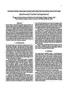
Amino acid sequence information has become available for hundreds of thousands of proteins in the last decade, owing to the advances in genome sequencing technologies. However, to understand the functional role played by each of these proteins in a cell, it is crucial to determine its structure, and as a first step, to determine its secondary structure. There are a class of proteins that reside embedded in the cell membrane, called membrane proteins. Parts of these proteins are found exposed to extra-cellular (ec) region and parts to the intra-cellular (cytoplasmic, cp) region, and there are segments that are embedded in the membrane (see Figure 1). These transmembrane (TM) segments are known to possess helical secondary structure for all plasma-membrane residing membrane proteins in eukaryotic organisms, and are characteristically different from nontransmembrane helical segments. Membrane proteins are present not only in the cellular membrane but also in membranes of organelles e.g. mitochondria, nucleus, endoplasmic reticulum.

1

0. Executive Summary

2

Figure 1: Schematic of cell and transmembrane and soluble proteins (A) The cell is enveloped by a cell-membrane (brown) and is surrounded by water medium (blue bubbles). The medium inside the cell is made of water as well (blue-pink). Soluble proteins are found completely inside the cell. Membrane proteins are partly embedded in the cell-membrane. (B) Transmembrane protein rhodopsin: It starts in the cytoplasmic region (top), traverses through the cell membrane to go into the extracellular region (bottom) and then traverses the membrane again to enter the cytoplasm. It has 8 helices, 7 of which are located mostly in the transmembrane region. (C) Soluble protein Lysozyme: The protein is immersed in an aqueous medium.

An introduction to proteins is presented in Chapter 2. The objective of this thesis is to develop computational approaches for the prediction of helical transmembrane segments in protein sequences. Accurately predicting one or more transmembrane segments in a protein in turn helps in identifying membrane proteins from soluble proteins. Focus of this work is on the more challenging problem of predicting transmembrane segments from only the primary sequence, as opposed to using evolutionary profile of the protein, in order to facilitate prediction even when such information is not available. Membrane proteins are a large fraction (∼25%) of all the proteins found in living organisms, and play vital roles in cellular functions such as signal transduction and transport of ions across the cell membrane. Knowledge of the transmembrane segment locations, boundaries and the overall topology of a membrane protein can 1. give insight into the function of the protein


3

2. be useful in narrowing down the possible tertiary structure conformations of the protein 3. help identify other proteins related to it in order to be able to apply any knowledge known about these proteins to the protein at hand 4. can be of use in drug-design by reducing the complexity of search between drugs and their target proteins. Experimental methods to determine the three dimensional structures of proteins such as NMR spectroscopy and x-ray crystallography are very tedious, and in case of membrane proteins, are often infeasible—transmembrane proteins aggregate in the absence of their natural hydrophobic environment, the membrane. The number of TM proteins with experimentally determined structure corresponds to only about 1.4% out of total protein structures deposited in the Protein Data Bank (PDB) as of early 2007 [1]. The importance of membrane proteins coupled with the difficulty in determining their structures by experimental methods, make it desirable and necessary to predict membrane protein structure by computational methods. The first questions pertinent to membrane protein structures are : 1. Is the given sequence that of a membrane protein? 2. How many transmembrane segments are present in this membrane protein? 3. What is the topology of this protein with respect to the cell membrane; namely, which of the non-membrane parts are inside the cell? and which are outside? 4. What are the boundaries of the transmembrane segments? The central component in addressing all of the questions is the identification of the locations of TM segments. Only subsequently, we can address the larger question of what are the tertiary contacts made between the amino acids in both the transmembrane and soluble portions of the protein.

3

Unsolved challenges — previous methods

There is no single method that can reliably determine the location and boundaries of transmembrane segments and the topology of the protein with respect to the cell membrane. This is primarily due to the following current limitations: 1. Limited representation of all possible structures in training data: Previous methods are limited by the fact that they are over trained to the limited available data, and thus are able to identify only those transmembrane proteins that have amino acid propensities similar to those of known transmembrane structure.


4

2. Previous “best” methods used stringent permissible topologies: The architecture of machine learning methods such as hidden Markov models which expect only a specific arrangement of transmembrane helices— that which is observed when the protein goes from one side of the membrane to the other side of the membrane before returning to the same side (such as shown in Figure 1). It is now known that this arrangement is not universal. A review of literature on computational methods for characterization and prediction of transmembrane helices is presented in Chapter 3 and Publication 2.

4

Models and methods: biological language modeling

The identification of transmembrane segments is a specific formulation of more general questions, namely “what are the building blocks of sequences” and “what do they infer about the structure or function of the sequence”. These questions are similar to those commonly asked pertaining to natural language texts — “what are common phrases in a language”, “what do they mean”. The specific question about transmembrane segments would correspond to a specific question in language, such as “does the style of text say something about the author”. This suggests that computational algorithms to address language related questions might be applicable to biology. The approach adopted in this thesis is to apply the concepts of language modeling to biological sequences. Specifically, the methods of statistical n-gram analysis, Yule’s word association measure and latent semantic analysis which are methods originally developed for text processing have been adapted to study biological sequences. Methods for adapting natural language processing algorithms to biological sequences are described in Chapter 4.

5

Datasets and metrics of evaluation

Analysis has been performed on benchmark datasets where available and also on “current” datasets available at the time of study. Metrics of evaluation are also standard methods used in literature. Datasets and metrics of evaluation for all the studies performed in this thesis are described in Chapter 5.


6

5

Biological feature development and analysis

At the outset, the thesis explores the biology-language analogy, and the applicability of algorithms from natural language processing (NLP) towards answering general questions pertaining to biological sequences. Subsequently, the observations and results are applied to the study of the specific problem of transmembrane helix prediction.

N-grams in biology Word n-gram statistical modeling is a very strong technique that captures many characteristics of language — characteristic style of an author, location of most meaningful content in a document or sentence. In the first part of this thesis, we applied the n-gram modeling techniques to biological sequences: 1. Biological Language Modeling Toolkit: First, a suite of tools called the Biological Language Modeling (BLM) toolkit has been developed to efficiently compute n-gram features of proteomic sequences. It preprocesses genome sequences into suffix arrays, and then computes n-gram features. More complex applications can be built over the functionality of the BLM toolkit. BLM toolkit is described in Publication 3 and the resulting collaborative work in Publication 4. 2. Identification of genome signatures: Analysis of most frequently occurring ngrams in one genome in comparison with the frequencies of these specific n-grams in other genomes lead to the identification of genome signatures. Further, amino acid neighbor preferences are different for different organisms. N-gram analysis of genome sequences are presented in Publication 10. 3. N-gram features in relation to protein structure and function: We explored if the n-gram idiosyncrasies coincide with the presence of functionally or structurally relevant information in proteins: • Folding. The locations of rare trigrams and experimentally determined folding initiation sites in the protein folding model system lysozyme were correlated. • Misfolding and Stability. Inverse n-gram frequencies were computed for two proteins and compared with the locations known to be important for their folding and stability of the protein. • Host-specificity of viruses. N-gram characteristics of specific viral proteins and the whole viral genomes were compared with the n-gram characteristics of the host species. • Negative charges in calcium sequestering proteins. N-grams have been computed to infer if high abundance of charged residues can identify calcium sequestering proteins.


6

In these examples, amino acid n-grams alone did not consistently identify the regions with maximum biological significance. In some cases, experimental data was not available to unambiguously establish the significance of the results. N-gram analysis of protein functions are presented in Publication 1. Computational analysis of misfolding and stability are described in Publication 6, but the n-gram analysis of the same are unpublished. 4. Other word-association features for protein structure prediction: In addition to n-grams, we also computed other related word association features, such as Yules association measure, and found them to capture characteristics distinguishing transmembrane helices from soluble helices. Yule’s association measure its application to soluble and transmembrane helices is described in Publication 11. Biological feature development through analysis employing n-gram and n-gram derived features are presented in Section 1 in Chapter 6.

Highly separable protein segment features using latent semantic analysis We borrowed a technique from NLP, latent semantic analysis (LSA). To quantitatively compare different types of vocabularies in their ability to capture biological meaning, we investigated several different vocabularies in a well known biological context. We chose a well defined biological problem, namely that of classifying protein secondary structural segments (helix, sheet and coil). The goal of this work was to: 1. Study the utility of different vocabularies in place of amino acids in characterizing different secondary structure elements. Three separate vocabularies were considered — (i) amino acids, (ii) chemical groups and (iii) amino acid types based on their electronic property. 2. Study if latent semantic analysis is useful for the problem of protein secondary structure prediction. We found that each vocabulary carried significant “meaning”, and that LSA is a very useful technique for biological sequence analysis. Feature analysis using latent semantic analysis for protein sequences is described in Sections 2 and 3 in Chapter 6 and in Publication 7.


7

7

Algorithm for transmembrane helix prediction

We then applied what we learnt from the studies described above to the challenging problem of TM helix prediction. Use of LSA for secondary structure classification established that alternate vocabularies contributed towards secondary structure prediction, and that types of secondary structure are better represented by different choice of vocabulary. Based on this, we chose to use all of the amino acid ↔ property mappings in conjunction with each other, for TM prediction. Specifically, we mapped amino acids to charge, polarity, aromaticity, size and electronic property, and constructed the LSA model over this expanded representation. The features of transmembrane and nontransmembrane segments constructed with this adaptation of LSA were very distinct from each other, indicating possibility of high accuracy of TM segment prediction. We systematically applied different feature extraction and prediction procedures making use of the observations from our approach of language modeling of protein sequences, and developed an algorithm for transmembrane helix prediction. We refer to this algorithm as TMpro. TMpro has been evaluated on the benchmark server and it outperformed the (previously) best of the sequence-alone methods, namely TMHMM v2.0 by 50% reduction in F-score. It is also very balanced between recall and precision of the helical segments. The Qok value, which indicates the number of proteins in which all segments are predicted correctly (with one-to-one correspondence to observed segments) is also higher by >10% w.r.t TMHMM. The strength of TMpro comes from the fact that it does not impose architectural constrains on the topology of the protein and does not overtrain the features to amino acid propensities observed, thereby allowing it to recognize more varied types of TM segments. On evaluating the methods on NR TM, a data set of nonredundant membrane proteins available today, TMpro achieves 20-30% reduction in segment error rate compared to the best of sequence-based prediction methods, and also outperforms in correctly distinguishing a larger number of membrane proteins from soluble proteins. Application of TMpro to specific proteins: To estimate TMpro’s ability to correctly predict TM helices in membrane proteins of unusual topology, KcsA and aquaporin, we applied TMpro to study these specific proteins. In both cases, TMpro performed favorably. TMpro was also used to predict TM structure in several membrane proteins with unknown structure. TMpro algorithm, performance evaluations, error analysis, error recovery, application to specific proteins and availability on a web server are described in Chapter 7 and in Publications 8 and 9.


8

8

Thesis contributions 1. A high accuracy method for TM helix prediction has been developed. It has been shown that it outperforms the current best methods, without any caveats of training data biases during evaluation. 2. Applicability of language analogy to address problems in biological sequence processing has been established through n-grams and latent semantic analysis and study of vocabularies. 3. TMpro has been applied to predict TM segments in proteins with unknown TM structure: PalH of Botrytis cinerea and glycoprotein GP41 of human immunodeficiency virus. Experimental studies to validate these predictions are underway. 4. The Biological Language Modeling Toolkit has been developed and released on the internet in open source1 at http://www.cs.cmu.edu/∼blmt/source/. 5. The TMpro algorithm has been made available on the web with novel features for analysis by expert biologists and computational scientists2 : http://linzer.blm.cs.cmu.edu/tmpro/.

Thesis contributions are summarized in Chapter 8 and future work is described in Chapter 9.

1

A web interface to the toolkit has been developed by Vijayalaxmi Manoharan with Dr. Judith Klein-Seetharaman and is available at: http://flan.blm.cs.cmu.edu 2 The web interface and web service have been developed in collaboration with Christopher Jon Jursa and Dr. Hassan Karimi, University of Pittsburgh School of Information Sciences

Chapter 1 Human Language and Biological Language: Analogies Genetic encoding has been referred to as a “language”, and a genome itself as “book of life” [2, 3, 4, 5]. Prior work established some characteristics that are similar between language and analogy: both follow the Zipf’s power law [6] of distribution of words which states that the rank of a word and its frequency are inversely related [7, 8]; a formal grammar is exhibited by biological sequence and structure [9, 10, 11]. Prior to this thesis, the linguistic characteristics exhibited by biological sequences have been established (mostly for DNA sequences), but little work has been done towards the application of computational language processing methods to solve specific questions pertaining to structure and function of biological sequences. The work presented in this thesis is the first systematic application of speech and language analogies to solve specific biological questions. Parallel to the work described in this thesis, there have been other applications of the language and speech analogy to biology [12, 13, 14, 13, 15, 16, 17].

1.1

Biology-text analogy

The analogy between language and biology is outlined schematically in Figure 1.1. 1. Understanding the structure and function of proteins strongly parallels the mapping of words to meaning in natural language processing. 2. The words in text documents map to a meaning, and combine in a linear fashion to convey information. Similarly, proteins may be seen as sequences of raw text which carry higher level information about the structure of the protein. Analysis of the text documents can give further higher level information about the topic and content of the text. Analysis of protein sequences gives information on protein-protein or protein-ligand interactions, and protein functional pathways. 9

1. Human Language and Biological Language: Analogies

10

Figure 1.1: Biology-language analogy

3. Availability of large amounts of text in digital form has lead to the convergence of linguistics with computational science, and has resulted in applications such as information retrieval, document summarization and machine translation. In direct analogy, transformation of protein science by data availability opened the door to convergence with computer science and information technology. Techniques used for natural language processing find significant applications to the study of relationships between biological sequences and their functional characteristics [12]. Aside of the results presented in this thesis (see Section 10), there are a number of other examples: linguistic complexity of DNA is used to detect repetitive regions and detect functionally important messages like transcriptional terminators [13] and to determine coding and non-coding region characteristics [18, 19]; text categorization towards protein classification [14]; and n-gram counts to study evolutionary relations between species [20]. Dictionaries of motifs that represent whole genome signatures or regulatory sites have been constructed [21]. Other examples for the use of linguistic approaches for bioinformatics can be found in refs. [22, 23, 24, 25, 26, 12, 13]. Recently, probabilistic language models have been used to improve protein domain boundary detection [15] and to predict secondary structure [16] and transmembrane helix boundaries [17].

1.2

Biology-speech analogy

Segmentation is an important step in speech analysis and applications. Below we discuss examples of speech tasks that have parallels in biology.


11

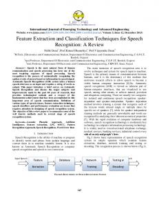
“Word” identification by signal recognition in proteins: In a spoken sentence, words are not separated from each other by spaces as in written text. Thus, automatic speech analysis and synthesis methods have to deal with identification of meaningful units. The task therefore shifts from statistical analysis of word frequencies to a stronger focus on signal identification and differentiation in the presence of noise. The task of mapping protein sequences to their structure, dynamics and function can also be seen more generally as a signal processing task. Just as the speech signal is a waveform whose acoustical features vary with time, a protein is a linear chain amino acids whose physicochemical properties vary with respect to position in the sequence. However, while a speech sample can take unlimited continuous values, or digitized values within a given digital resolution, for proteins the value can be only one out of the possible twenty amino acids or a few possibilities of their physicochemical properties. The goal of speech recognition is to identify the words that are spoken. There are several hundred thousand words in a typical language. These words are formed by a combination of smaller units of sound called phones. Recognizing a word in speech amounts to recognizing these phones. There are typically 50 phones in speech. For protein sequences, there are motifs of secondary structure, the secondary structure elements itself and subpatterns in the secondary structure elements (helix cap, helix core, etc). Thus, identification of structural elements in protein sequences using the signal processing approach is equivalent to phone recognition. Application of speech analogy to transmembrane proteins: Identifying the differences between membrane and soluble secondary structure elements is analogous to the analysis of speaker variability in the signal processing field. Consider the signal characteristics of a word spoken by two different persons, especially if one is female and the other is male. Although the fundamental nature of the sounds remains the same, the overall absolute values of the signal composition are different. For example, a vowel sound has the same periodic nature, but the frequency is different. See the frequency compositions of the same sentence spoken by a male and a female speaker shown in Figures 1.2A and B. Identifying the phones alone is not sufficient. The content of a speech signal is not dependent on the signal alone; its interpretation relies on an external entity, the listener. For example, consider the phrases: - How to recognize speech with this new display - How to wreck a nice beach with this nudist play The speech signals or spectrograms showing the frequency decomposition of the sound signals for these two phrases spoken by the same speaker are shown in Figures 1.2B and 1.2C. The two very different sentences are composed of almost identical phone sequences. In this example, finding out which of the two sentences was uttered by the speaker cannot be determined from the spectrogram alone, but depends on the context in which it was


12

spoken. Thus the complete information for interpretation is not contained in the speech signal alone, but is also inferred from the context. In contrast, the linear strings of amino acids that make up a protein contain in principle all the information needed to fold into a 3-D shape.

Figure 1.2: Spectrograms of the same sentence spoken by different speakers The x-axis shows progression of time and the y-axis shows different frequency bands. The energy of the signal in different bands is shown as intensity in grayscale values with progression of time. (A) and (B) show spectrograms of the same sentence “How to recognize speech with this new display” spoken by two different speakers, male and female. Although the frequency characterization is similar, the formant frequencies are much more clearly defined in the speech of the female speaker. (C) shows the spectrogram of the utterance “How to wreck a nice beach with this nudist play” spoken by the same female speaker as in (B). (A) and (B) are not identical even though they are composed of the same words. (B) and (C) are similar to each other even though they are not the same sentences. See text for discussion.

The analogy of speaker variability in the protein world can be found in the categorization of proteins into soluble and membrane proteins. In contrast to soluble proteins, which are entirely immersed in an aqueous environment, membrane proteins have some segments that are located in an aqueous environment, while other segments are located in a chemically different environment, the membrane lipid bilayer, as shown in Figure 1C. Since the environment differs for different segments in TM proteins, the chemical and physical characteristics displayed by these segments are also different. TM helix


13

prediction is closely related to protein secondary structure prediction given the primary sequence. Secondary structural elements such as helix, strand, turn and loop are still the basic components of the three dimensional structure of membrane proteins; however their characteristics are different from those of the soluble proteins when they are located in the membrane embedded parts. This difference, or localization-variability, may be seen as the speaker variability in speech. The soluble and TM segments can be thought of as speech that is spoken by two different speakers, or three different speakers if the soluble portions are further separated as extracellular and cytoplasmic soluble portions. Signal processing methods have been used for decades to capture the nuances of speech signals for speech and speaker recognition (see for example [27]). Despite the power of these mathematical tools of signal processing, their application to protein sequences has been minimal to date. The few instances where these methods have been applied are reviewed below. One of the very first applications was in the computation of the hydrophobic moment of protein domains [28] and in detecting periodicities in secondary structure (α-helix, βsheet and 310 -helix) [29]. Wavelet analysis of the hydrophobicity signal has been used to locate the secondary structure content relating the periodicity observed in the signal to the known values of secondary structure period [30]. This is based on the fact that the period of a helix is 3.6 residues, that of a sheet is 2 to 2.3 residues and that of a 310 helix is 3 residues [29]. In another application of signal processing technique, Fourier transformation was used to extract the sequence periodicities to classify structural motifs into different architectures. To this end, the Fourier spectrum is computed from the hydrophobicity and secondary structure signal of a proteins, and the power spectrum served as the feature input into a neural network [31]. Last but not the least, hidden Markov modeling, used extensively for computational biology applications such as sequence comparison, was originally applied for speech processing applications [32]

1.3

Computational Methods for Language and Speech Processing

In this chapter we present an introduction to algorithms in computational natural language processing or speech or speaker recognition that we applied to biological sequences in this thesis work. Detailed references for these fields are the books by Manning and Schutze [33] and Rabiner and Juang [34].

1.3.1

N-grams

N-grams refer to sequential occurrences of n words in a text. For example, the following 3-grams may be seen in the sentence A party was thrown because Congress party has won the General Elections, a party was, party was thrown, was thrown because, · · ·


14

· · ·, Congress party has, party has won, · · · For languages where a word-level dictionary is available but not computational parsers of the grammatical phrase-structure of the text, “frequency counts” of the n-grams in the texts can reveal the “meaningful content” of the text. For example, the word party has multiple meanings, two of them being (i) a social get-together and (ii) a group of people involved in some political activity. Construction of 3-gram counts from texts pertaining to different topics, or in other words, making a 3-gram language model of different collections of texts, it is possible infer that in the first occurrence, the word party refers to the first meaning and the second occurrence refers to the second meaning. Language technologies often use word n-grams as features to study characteristics of texts. N-grams are used in information retrieval, author recognition, plagiarism detection and word sense disambiguation.

1.3.2

Yule’s q-statistic

Yule’s q-statistic (henceforth called Yule value) is a correlation measure between two words [35]. It is used to infer from the presence or absence of a word, likelihood of finding another word. It takes a value between +1 and -1 corresponding to the range of “either both words are present or both words or absent” to “if one occurs, the other does not occur”. For example, the word pair protein and phone would have a Yule value close to -1, whereas the word pair protein and nutrition would have a positive value such as 0.6. Traditionally, in natural language processing, the Yule value is computed over windows of a specific length, and a word pair is said to appear together if both the words appear in the window, irrespective of which position they appear in. For example, for a window size of 6, the word pair new and car are said to occur together irrespective of whether the text is new car or new blue car or new light blue car. The Yule value Yd (x, y), for a pair of words x and y within in a window of a length d is given as Y (x, y) =

N00 N11 − N01 N10 N00 N11 + N01 N10

(1.1)

N11 is the number of windows in which both the words x and y occur N00 is the number of windows in which neither of the words occur N10 is the number of windows in which word x occurs but not word y N01 is the number of windows in which word x does not occur but not word y occurs

1.3.3

Latent semantic analysis

A mathematical framework that can capture synonymy of words, is latent semantic analysis (LSA) [36]. Text documents are represented as bags-of-words, that is, as a vector of counts of all the words in the vocabulary.


15

Latent semantic analysis is performed on a collection of text documents, to infer similarities between the documents based on the similarities of distribution of words between the documents. It has the capability to infer contextual similarity of words based on their collocations across the given corpus, and hence it can recognize ‘latent’ similarities between documents when they share similar but not identical words. Vocabulary: A list of all the unique words in the corpus is created, after removing stop words (e.g., the, a, are, on, of, . . . ) and after stemming (i.e, taking only the root of the word, e.g., stemmed version of the words talking, talked, talk is talk. This final list of words after stop word removal and stemming is referred to as vocabulary of the document collection. Word-document matrix: A large matrix is created, in which rows are labeled by the different words in the vocabulary and the columns are labeled by documents in the corpus. The cell Cij in the matrix corresponding to the ith row and j th column contains the number of times the ith word appears in the j th document. Let the total number of documents be N ; let V be the vocabulary and M = |V | be the total number of words in this vocabulary. Each document di can then be represented as a vector of length M : di = [w1i w2i ... wM i ] (1.2) where wji is the number of times word j appears in the document i, and is 0 if word j does not appear in it. The entire corpus can then be represented as a matrix formed by arranging the segment vectors as its columns. The matrix would have the form W = [wji ], 1 ≤ j ≤ M, 1 ≤ i ≤ N

(1.3)

The information in the document is thus represented in terms of its constituent words; documents may be compared to each other by comparing the similarity between the document vectors. The absolute word counts are clearly related to the length of the segment and also to the overall distribution of that word in all of the corpus. To compensate for the differences in document lengths and overall counts of different words in the document collection, each word count is normalized by the length of the document in which it occurs, and the total count of the words in the corpus. This representation of words and documents is called vector space model (VSM). Documents represented this way can be seen as points in the multidimensional space spanned by the words. Singular value decomposition: In order to capture the latent similarity between the documents, the matrix is subject to singular value decomposition (SVD) [37]. The matrix W is decomposed into three matrices by SVD and they are related as W = U SV T

(1.4)


16

where U is M × M , S is M × M and V is M × N (recall that M is the number of words in the original matrix and N is the number of the documents, that is, the dimension of the matrix W is M × N ). U and V are left and right singular matrices respectively. SVD maps the document vector into a new multidimensional space in which the corresponding vectors are the columns of the matrix SV T . Matrix S is a diagonal matrix whose elements appear in decreasing order of magnitude along the main diagonal and indicate the energy contained in the corresponding dimensions of the M -dimensional space. Normally only the top R dimensions for which the elements in S are greater than a threshold are considered for further processing. This is achieved by setting sjj ∀j > R

(1.5)

Thus, the matrices U , S and V are reduced to M × R, RxR and R × N , respectively, leading to a data compression and noise removal. The space spanned by the R vectors is called eigenspace. Classification: Given a corpus of documents and their topics, the goal is typically to identify the topic to which a new document belongs. A metric of “relatedness” between documents such as the cosine similarity is defined below. Classification methods (Knearest neighbor, support vector machine, etc) are used to determine which of the training documents the new document is most similar to. The topic of the new document is assigned as that of the similar document. Cosine similarity: This is the measure used in determining the similarity between two document vectors. For two vectors X = [x1 x2 xN ] and Y = [y1 y2 yN ], the cosine similarity is defined as cos(X, Y ) =

1.3.4

x1 y1 + x2 y2 + + xN yN |X|.|Y |

q

where, |X| =

x21 + x22 + + x2N

(1.6)

Wavelet transform

The first step in signal processing is usually the application a mathematical transform that can identify periodicities and variations in signals even in the presence of background noise. The ability to identify periodicity is applied to for example, pitch-detection in speech or to edge-detection in images. Wavelets are functions ψ(t) that can analyze a time-series signal at different scales or resolutions, and are used to locate patterns in the signal. If we look at a signal, say p(t), through a large “window”, we identify gross features; if we look at the same signal with a small “window,” we differentiate detailed features. Wavelet analysis is designed to see the forest and the trees. A wavelet is a waveform that is localized in both time (or space) and frequency domains. A variety of different wavelet shapes have been used, of which three commonly used shapes are shown in Figure 1.3. These are (i) First derivative of


17

Figure 1.3: Wavelets Three examples of analysis wavelets are shown: 1st derivative of Gaussian, Mexican Hat and Morlet wavelets, from left to right. 1st derivative of Gaussian (left) is anti-symmetric to the center, and is suitable to identify step-up or step-down nature of an input signal. Mexican hat (middle) is a symmetric wavelet with a single peak. Morlet wavelet (right) is also symmetric but is characterized by multiple peaks and is more suitable to capture ripples or multiple cycles of a periodic signal.

Gaussian, (ii) second derivative of Gaussian, called the Mexican Hat, and (iii) the Morlet wavelets. The underlying function ψ(t) for the Mexican hat wavelet is shown in Equation 1.7 as an example [38]. t2

ψ(t) = (1 − t2 )e− 2

(1.7)

The transformation of a time-series signal p(t) using wavelets is performed as follows. The wavelet ψ(t) is convolved with the time-series signal p(t) to obtain its wavelet coefficients. This amounts to translating the wavelet to a position in the signal, and computing the product-sum of the wavelet and the signal, which would be the value of wavelet coefficient at that position. The process is repeated by translating the wavelet to all the positions of the input signal, and thus obtaining wavelet coefficients at all these positions. The original wavelet is called the mother wavelet or the analyzing wavelet. The mother wavelet is then scaled, a process referred to as dilation. The dilated wavelet is referred to as child wavelet. Wavelet coefficients are computed again with the child wavelet, where the child wavelet has been obtained by dilating the mother wavelet to scale a. The complete set of wavelet analysis functions in dependence of translation factor b and dilation √ factor a is given by Equation 1.8 [38]. A normalizing factor 1/ a is used to maintain the energy constant in the wavelet at all scales. Ã

1 t−b ψ(a,b) (t) = √ ψ a a

!

(1.8)

To illustrate, a set of mother and child wavelets for the Mexican Hat function are shown in Figure 1.4. The effect of dilation (by varying the dilation factor a) is shown in the top panel of the figure, and the effect of translation (by varying the translation factor b) is shown in the bottom panel of the figure. In each case, the mother wavelet is shown


18

Figure 1.4: Mexican hat wavelet at different dilations and translations The mother wavelet of Mexican hat is shown in bold in both (A) and (B). In (A), Dilation factors a = 2 and a = 4 are shown in grey shade, when translation is zero (b = 0). In (B) the translated wavelets of the mother wavelet are shown at b = −5 and b = 5.

in bold. Specifically, Figure 1.4 (top panel) shows the Mexican hat mother wavelet with a = 1, along with the dilated wavelets at scales a = 2 and a = 4. Figure 1.4 (bottom panel) shows the mother wavelet in bold at translation b = 0, and translated to positions b = −5 and b = 5. Finally, the wavelet transform of a given signal p(t) with respect to the analyzing function (t) is computed as defined in Equation 1.9 [38]. Ã

!

1 Z∞ t−b T (a, b) = √ dt p(t)ψ ∗ √ a −∞ a

(1.9)

where, a is the dilation or scale, b is the translation, and ψ ∗ represents complex conjugate of ψ. Note, that in the case of the Mexican hat, the wavelet function ψ(t) is a real-valued function, whereby ψ(t) = ψ ∗ (t).

1.4

Application to biological sequences

Application of n-gram analysis to biological sequences: In biological sequences, the best equivalent of words is not known. Thus, n-grams usually describe short sequences


19

of nucleotides or of amino acids of length n. The distributions of n-grams in genome sequences of individual organisms have been shown to follow Zipf’s law [39, 40, 41, 41, 7, 8, 42, 18, 43, 11]. Other “vocabulary” that has been used includes the 61-codon types, or reduced amino acid alphabets [44, 45, 46, 47]. Prior to this thesis, N-grams were not applied to address any specific biologically relevant question about the organism. BLAST algorithm for sequence alignment ([48]) and Rosetta protein tertiary structure prediction algorithm [49] can both be viewed as applications of n-grams, albeit they are not “analogous” to how n-grams are used in language technologies. Application of Yule’s q-statistic or latent semantic analysis to biological sequences: Yule’s q-statistic and LSA have not been applied to biological sequences prior to this work. Application of wavelets to biological sequences: Wavelets have been used in place of a simple window (triangular or trapezoidal) to smooth the hydrophobicity signal to make predictions on the location of membrane spanning segments [50, 51]. Following this work, wavelet transforms have been applied for transmembrane helix prediction but the application has primarily been only to smooth the hydrophobicity signal by removing high frequency fluctuations [52, 53, 54, 55]. The other application of wavelets to protein sequences is to compare sequence similarity of proteins based on correlation between their wavelet coefficients [56].

Chapter 2 Introduction to Proteins Proteins are complex molecules that carry out most of the important functions in the living organism—signal transduction, transport of material, defense of self from foreign bodies, are all functions carried out by thousands of different proteins in the body. Proteins also play structural roles such as forming tissues and muscular fiber. Interactions between proteins mediated by their structures form the fundamental building blocks of functional pathways in living organisms. In this chapter we present an introduction to proteins. For an in depth understanding of proteins, refer to the textbook [57].

2.1

Amino acids: primary sequence of proteins

Proteins are made up of amino acids. These amino acids are linked to each other in a linear fashion like beads in a chain, resulting in a protein (see Figure 2.1). There are 20 different amino acids, all of which share a common chemical composition (Figure 2.1A). There is a carbon atom called Cα at the center, which forms 4 covalent bonds—one each − with (i) amino group (NH+ 3 ), (ii) carboxyl group (COO ), (iii) hydrogen atom (H) and (iv) the side chain (R). The first three are common to all amino acids; the side chain R is a chemical group that is different for each of the 20 amino acids. Figure 2.1B shows the side chains of the 20 amino acids along with their names and the 3-letter and 1-letter codes commonly used to represent them. In most of the computational methods, the amino acids are commonly represented by the 1-letter code: A, C, D, E, F, G, H, I, K, L, M, N, P, Q, R, S, T, V, W, Y. Two amino acids can join to each other through condensation of their respective carboxyl and amino groups, shown schematically in Figure 2.1C. The oxygen (O) from the carboxyl group on the left amino acid and two hydrogen atoms (H) from the amino group on the right amino acid get separated out as a water molecule (H2 O), leading to the formation of a covalent bond between the carbon (C) and nitrogen (N) atoms of the carboxyl and amino groups respectively. This covalent bond, which is fundamental to all proteins, is called the peptide bond. The peptide bond is shown in violet color in Figure 2.1C. The carboxyl group of the right amino acid is free to react with another amino 20

2. Introduction to Proteins

21

Figure 2.1: Amino acids (A) Amino acid: there is a carbon atom at the center (Cα (yellow)) that forms 4 covalent bonds with: amino group (blue), carboxyl group (red), hydrogen atom (green) and the side chain R (pink). (B) There are 20 possible side chains giving rise to 20 amino acids. The names of the 20 amino acids and their 3-letter and 1-letter codes are also shown. (C) A covalent bond (called peptide bond) can form between the carboxyl group of one amino acid and amino group of the other, there by releasing one water (H2 O) molecule. (D) Carboxyl group of the second amino acid is free to make a peptide bond with a third amino acid, thus forming a chain of amino acids called a peptide or a protein


22

acid in a similar fashion. The Cα H along with the N, C, O and H atoms that participate in the peptide bond, forms the main chain or back bone of the protein. The side chains are connected to the Cα atom. The progression of the peptide bonds between amino acids gives rise to a protein chain. A short chain of amino acids joined together through such bonds is called a peptide, an example of which is shown in Figure 2.1D. Synthesis of proteins in cells happens in principle in the same fashion outlined above, by joining amino acids one after the other from left to right; in the cells, each step in the formation of a protein is controlled by other enzymatic proteins. Conventionally, a protein chain is written from left to right, beginning with the NH+ 3 (amino) group on the left and ending with the COO− (carboxyl) group on the right (same as in Figure 2.1C). Hence, the left end of a protein is called N-terminus and the right end is called C-terminus. The term “residue” is commonly used to refer to any amino acid in the protein sequence.

Amino acid properties The 20 amino acids have distinct physical and chemical properties because of the differences in their side chains. Many different criteria for grouping amino acids based on their properties have been proposed. Several hundred different scales relating the 20 amino acids to each other are also available (e.g. see [58], [59]). The major difficulty in classifying amino acids by a single property is the overlap in chemical properties due to the common chemical groups that the amino acid side chains are composed of (chemical groups that all 20 amino acid chains are composed of are shown in Figure 2.2).

Figure 2.2: Chemical groups Left panel shows examples of amino acid side chains, and the individual chemical groups that are constituents of the side chain. Right panel shows all the individual chemical groups that the 20 amino acids are made of.

Some commonly used properties and the set of amino acids that share the respective property are shown in Table 2.1.


Vocabulary Charge

Polarity Aromaticity

Size

Electronic Property

Words

23

Symbols

Positive Negative Neither Polar Nonpolar Aromatic Aliphatic Neither Small Medium Large Strong donor Weak donor Neutral Weak acceptor Strong acceptor

p n . p n R . . o O D d a A

Amino acids H, K, R E, F ACDGILMNPQSTWY CDEHKNQRSTY AFGILMPVW ILV FHWY ACDEGKMNPQRST AGPS DNT CEFHIKLMNQRVWY ADEP ILV CGHSW FQTY KNR

Numeric value +1 -1 0 1 0 / -1 +1 -1 0

+2 +1 0 -1 -2

Table 2.1: Amino acid properties Different types of vocabularies used are shown in column 1. For each type, all the words in the vocabulary and the amino acids mapping to these words are listed in columns 2 and 4. Column 3 lists the symbol used in place of the corresponding word.

Three amino acids, namely cysteine, proline and glycine, have very unique properties. Cysteine contains a sulphur (S) atom, and can form a disulphide covalent bond with the sulphur atom of another cysteine. The disulphide bond gives rise to tight binding between these two residues and plays an important role for the structure and stability of proteins. Similarly, proline has a special role because its backbone is a part of its side chain structure. This restricts the orientation of the peptide around a proline, and usually gives rise to a turn or kink in protein structures. Glycine has an opposite effect in a peptide, since it has a side chain that consists only of one hydrogen atom (H). Since H is very small, glycine imposes much less restriction on the polypeptide chain than any other amino acid.

2.2

Secondary structure

Inspection of the three dimensional structure of proteins reveals the presence of repeating elements of regular structure, termed secondary structure (compare Figures 2.3 A and B). These regular structures are stabilized by interactions between atoms within the protein,


24

Figure 2.3: An example to demonstrate the primary, secondary and tertiary structure of proteins (A) The structure of the protein Lysozyme (Protein Data Bank code 1HEW) is shown. The backbone is shown in ball and stick model in rainbow colors from one end to the other end; side chains are shown in grey. The sequence of amino acids that make up this protein is called its primary sequence or primary structure. (B) The backbone is superimposed with ribbons to highlight the folds in the protein. The overall three dimensional structure of the protein is called its tertiary structure. (C) On closer observation of the structures of proteins, three types of repetitive structures that are ’localized in 3D space’ are observed, and they are: helix (red), sheet (yellow) and loop (blue). These are referred to as secondary structures because they form the intermediates between primary sequence and the final tertiary structure of the protein.

in particular the Hydrogen Bond. Hydrogen bonds are non-covalent bonds formed between two electronegative atoms that share one H. There is a convention in the nomenclature designating the common patterns of hydrogen bonds that give rise to specific secondary structure elements, the Dictionary of Secondary Structure in Proteins (DSSP) [60]. Helix, is the secondary structure formed due to hydrogen bond formation between the carbonyl group of ith residue and the amino group of the i+nth residue, where the value of n defines whether it is a 310 , α or π helix for n = 3, 4, 5 respectively. Therefore, the interactions between amino acids that lead to the formation of a helix are local to the residues within the helix. Sheets on the other hand, form due to long-range interactions between amino acids, that is, residues i, i + 1, ..., i + n form hydrogen bonds with the residues i + k, i + k + 1, ..., i + k + n (parallel beta sheet), or in the reverse order with i + k, i + k − 1, ..., i + k − n (anti-parallel beta sheet). A turn is defined as a short segment that causes the protein to bend. A coil is that segment of the protein that does not conform to any of the secondary structure types just described. Typically, the seven secondary structure types are reduced to three groups, helix, (includes types α−helix H and 310 −helix G), strand (includes β− sheet) and coil (all other types). Figure 2.3C shows the secondary structure types helix, strand, turn and coil in different colors. The linear sequence of amino acids that the protein is made up of, is referred to as


25

the primary sequence or primary structure. The description of which parts of the protein assume which secondary structure type, namely helix or sheet, is referred to as the secondary structure (see Figure 2.3). A complete information of the 3-dimensional positions of all atoms in the protein, or a description of how the secondary structure motifs fold to form specific domains, is referred to as tertiary structure. The arrangement of multiple proteins (multimers), stably associated with each other, is referred to as the quaternary structure. Though some proteins exist as monomers, it is very common for proteins to form multimers. Figure 2.4B is an examples of a multimers. The quaternary structure can formed from identical or nonidentical protein chains.

2.3

Tertiary structure and structure-function paradigm

Figure 2.4: Protein function is exerted through its structure A. Lysozyme (PDB code 1HEW). The protein is colored in rainbow color from one end to the other end. Its structure create a groove which can dock its ligand shown in magenta color. B. Potassium channel (PDB code 1BL8. The helical segments in this multimeric protein form a vertical bundle, holding loop regions that line a pore. The sidechains of the residues on the loop act as selectivity filter for potassium ions that are allowed to pass through the pore.

Proteins play functional and structural roles in living organisms. Functional roles include transduction of sensory or electrochemical signals (example G-protein coupled receptors), enzymatic action (example lysozyme), defense against foreign bodies (example antibody), transport (example heomoglobin), regulation (hormones, ion channels and transcription factors). Structural roles are played proteins contributing to the structure or stability of a cell body (example integrins). A crucial task of a protein in the process of


26

exerting its function is recognizing a specific molecule out of the thousands of molecules it may come in contact with. Each protein has the ability to recognize a designated molecule, possibly another protein. This is achieved through interactions between atoms in one protein with atoms in other proteins or molecules. The molecule that a protein binds to is called a ligand. The three dimensional structure of the protein creates a suitable surface of potentials by which interactions with other molecules can take place; this structure is well defined for most proteins, although many proteins may posses multiple alternate structural conformations, and these may be responsible for different functional states. Figure 2.4 shows two examples of how the three dimensional structure of a protein allows it to perform its function. Figure 2.4(A) shows the enzyme Lysozyme in rainbow color demonstrating how its three dimensional structure creates a prominent cleft between its two domains. The ligands that dock into this cleft are bacterial cell wall proteoglycans. Lysozyme hydrolyzes its ligands and leads to breakdown of the bacterial cell wall. Thus, the three dimensional structure of lysozyme enables it to function in self defense. Figure 2.4(B) shows an ion-channel. It has a multimeric arrangement of 4 identical protein chains (only two of which are shown in the figure for clarity). Each chain consists of two helices, and the residues on its loop create a selectivity filter allowing passage of only K+ ions through the channel. The protein is not only selective of the specific ions it allows to pass through, but can also change between open and closed conformations of the pore [61].

2.4

Membrane and soluble proteins

Most of the proteins in an organism are present inside the cell, which is made mostly of water. Proteins that are completely in water are called soluble proteins. In contrast, some proteins are embedded in the membrane enveloping the cell, and these are called membrane proteins. The cell membrane is made up of hydrophobic fats and lipids, and provides a different environment compared to the polar aqueous (water) environment in the cell (Figure 1) than soluble proteins. Membrane proteins have a significant portion embedded in the cell membrane, and therefore experience a different environment (Figure 1B). The cell membrane is 30 ˚ A thick, and consequently a TM helix that spans the membrane is at least 19 residues long. In cases where the TM helix is embedded obliquely in the membrane, it may be longer than 19 residues. On an average, TM helices are 22-25 residues long. About 20-30% of genes in an organism encode membrane proteins [62, 63]. These proteins play important roles in signal reception and in physical and electrochemical interactions of cells with their environment [64, 65, 66, 67]. For example, ion channels mediate electrochemical transfer across the cell membrane by opening and closing of a pore [68]. G-protein coupled receptors (GPCRs) which form the single largest family of proteins with over 1000 genes encoding them in human genome [69] are also membrane proteins which react to a large and diverse set of ligands. Many environmental signals such as light and smell initiate signal transduction pathways through conformational changes


27

in GPCR structure [70]. 50% of all contemporary medicines are designed to act on this single family of membrane proteins, the GPCRs [71].

2.5

Membrane protein families and function

Many proteins are related to each other through evolution from bacterial organisms to humans. Many of the fundamental functions of cells, such as genome replication are carried out in part by proteins that are conserved in all organisms. Conservation can be detected by sequence similarity. When two proteins share the same evolutionary origin, they will likely conserve the identity or property of these amino acids crucial to protein structure and function in a given context. In some cases, however, there have been so many changes during evolution, that a common ancestry cannot be established unambiguously. In such cases it is also possible that the same structure and function has evolved independently. For example, the three dimensional structure of human rhodopsin, a protein in visual system that reacts to light, is similar to that of bacteriorhodopsin, a protein that acts as a proton pump in archaebacteria. Proteins that have similar three dimensional structure are said to come from the same superfamily. It is possible for proteins from the same superfamily to possess unidentifiable sequence similarity. If proteins from the same superfamily do possess sequence similarity they are said to come from the same family.

Figure 2.5: Topologies of membrane proteins (A) Rhodopsin. Green color shows transmembrane regions. (B) KcsA potassium channel. (C) Aquaporin (shown in rainbow color to highlight two short helices, each of which has flanking loops that exit on to the same side of the membrane).

In the alpha-helical class of transmembrane proteins that is of interest in this thesis,


28

there are 40 known superfamilies and 52 families spanned by 123 unique protein structures known till 2006 (OPM database 1.1 release date March 2006) [72]. All helical membrane protein families contain transmembrane helices, but their numbers, lengths and orientations differ. Most membrane proteins studied to date conform to a common arrangement of each of the transmembrane segments (Figure 2.5A). First, the transmembrane segments are long enough to span the thickness of the membrane, typically longer than 19 residues. Secondly, the transmembrane helices have their two ends on two different sides of the membrane (in other words, the topology of the protein alternates as . . . ec-TM-cp-TM-ec . . .). This topology was believed to be typical of all transmembrane helical proteins until recently. Superfamily structures determined in recent years, like those of voltage-gated channel like proteins, chloride channel like proteins and major intrinsic proteins (aquaporin-like proteins) revealed that the transmembrane helices can be as short as 8 residues and that the flanking loops of a transmembrane segment can be located on the same side of the membrane (see Figure 2.5B and C). This paradigm shift makes a significant impact on the design of computational methods for transmembrane helix prediction. Most of the earlier methods are based on the previous model of expected transmembrane topology, and methods that take into account the new possible topologies are only beginning to emerge (see Chapter 3).

2.6

Proteomes

The collection of all the proteins expressed in an organism at a time is referred to as the proteome (this also captures the quantity of a given protein expressed at that time). Variations of the term are also used, for example to say membrane proteome, referring to only membrane proteins, or cellular proteome referring to proteins expressed in one cell type, and the organism proteome, which refers to the set of all unique proteins belonging to the organism, namely the protein equivalent of the genome of the organism. To give an estimate, the human genome for example includes about 25000 genes that encode for one million different proteins according to the Human Proteome Initiative [73]. In the work in this thesis, the terms proteome and whole genome refer to the organism proteome.

Chapter 3 Literature Review in Transmembrane Helix Prediction A first step towards developing a transmembrane (TM) helix prediction algorithm is the understanding of the characteristics of TM helices that might help in distinguishing them from background information and specifically from non-TM helices. The 30 ˚ A thick hydrophobic lipid bilayer suggests that the TM helices are made up of contiguous hydrophobic residues, but exceptions exist: a long hydrophobic stretch may be a buried helix in a globular protein, or a TM segment may sometimes not be completely hydrophobic if it is shielded from the cell-membrane by interaction with other TM segments in the protein. In this chapter we review the previous methods for transmembrane helix prediction. We describe segment-level and residue-level distinctions between transmembrane segments and soluble or nontransmembrane segments, followed by algorithms for prediction of transmembrane helices.

3.1

Segment-level distinctions between transmembrane and soluble helices

TM helices are characteristically different from helices in globular domains of soluble or membrane proteins in several aspects, summarized below. TM helices are longer: On an average TM helices are longer compared to soluble helices — average length of TM helices is 23 residues and they are typically larger than 19 residues, while the average length of soluble helices is 9 residues [74]. Average hydrophobicity of TM helices is much higher: Average hydrophobicity of TM helices is much higher than that of soluble helices; in one study, close to half of the analyzed TM helices were more hydrophobic than any of the soluble helices analyzed 29

3. Literature Review in Transmembrane Helix Prediction

30

even when soluble helices of only comparable length of a minimum of 19 residues were included in the study [75]. However, about 25% of the ‘most-hydrophobic segment’s in membrane proteins had same range of hydrophobicity as that exhibited by soluble helices [75] indicating that some of the TM segments may not be distinguishable from soluble helices based on hydrophobicity alone. Polar or charged residues are buried in TM helices: The few polar or charged residues in TM helices are usually buried in the interior of helical bundles. In contrast, polar and charged residues in soluble helical bundles usually face the outside, while hydrophobic amino acids form the buried core [76, 77]. This observation is referred to as inside-out rule. Another study showed however that the charged or polar residues Q, K and R can be lipid facing. It is assumed that the reason for this is that these residues have long side chains which can snorkel towards the membrane surface interact with the lipid polar head groups [74]. TM helix bundles pack more tightly with each other: TM helix bundles pack more tightly with each other than do the soluble helix bundles, based on a study of contact plots and occluded surfaces ([78, 79] and their previous work). This also means that the residues on the helix-helix interaction faces (buried faces) are small and polar contributing to the tight packing. A significant observation in this context is that glycine which is known to be a helix breaker in soluble helices is found with a higher propensity in TM helices than expected because they provide opportunities for tight packing according to the “knot- into holes” concept [80]. Proline has a high packing value in membrane proteins: Proline has a high packing value in membrane proteins but a low packing value in soluble proteins where it is known to act as a helix breaker. Kinks and bending motions are more often observed in helices which contain more than one proline PxxP or a combination of proline and glycine PxxG, spaced four residues apart [81]. Two other specific motifs are found abundantly in membrane helix bundles, giving rise to a tighter packing of the helices. One motif is the leucine zipper motif LxxLxxxLxxL which is also found in soluble helix bundles. The other motif is the glycine motif GxxxG which is common to only membrane helices [78, 82] and references therein).

3.2

Residue-level propensities of amino acids

A number of amino acid propensity scales have been calculated through statistical analysis of residues in known TM and non-TM regions. 222 published amino acid indices were compared through cluster analysis by [83], of which 88 were different hydrophobicity scales alone.


31

Hydrophobicity: Hydrophobicity of a residue was first defined in terms of its chemical structure. Many other scales have been computed later through statistical propensities of amino acids in transmembrane and nontransmembrane regions. The most commonly used hydrophobicity scales are those derived by Kyte and Doolittle [84], Engelman et al [85], Jones et al [86] White and Wimley [87, 88], and Deber et al [89]. White and Wimley used a thermodynamic framework to experimentally measure and model the energetics of interactions of peptide chains with the lipid bilayer. Unlike previous methods of computing hydrophobicity of amino acids which take into account only the hydrophobicity of side chains and do not include the peptide bond contributions, they compute the free energy change associated with the partitioning of peptide from water into membrane as a result of multiple processes-hydrophobic effect, electrostatic attraction between amino acid residues and anionic lipids, loss of degrees of freedom due to immobilization in the membrane and the perturbation of the lipid due to the insertion of the peptide [87, 88]. A propensity scale is derived from this analysis [90], which has shown to be better than previous methods for characterization of characterization of transmembrane segments. A number of hydrophobicity scales have been devised:1 A-cid and Av-cid [91], BenTal el al (unpublished), Bull-Breese [92], Fauchere [93], Heijne [94], Hopp-Woods [95], KD [84], Lawson [96], Levitt, [97], Nakashima [98], Radzicka [99], Roseman [100], Sweet [101], Wolfenden [102] and WW [103]. Other Scales: A scale called the knowledge based scale for propensity of residue orientation in TM segments (kPROT) has been derived by analyzing a database of single and multi-spanning TM segments [104] for these three segments of membrane spanning helices (centre, extracellular-end and cytoplasmic-end). Jones et al observed that TM segments are often amphipathic when the protein has multiple membrane spanning segments and computed amino acid propensities separately for five classes of topogenic locations: membrane-outside, membrane-inside, membrane-middle, loop-outside and loopinside, and also separately for single-spanning and multi-spanning proteins. The scales are computed based on a data set of 83 integral membrane proteins [86]. Charge: A lipid accessibility scale that accounts for many factors influencing the amino acid propensities in different locations in the membrane segment as opposed to water solubility alone, is derived by a careful study of membrane proteins with known structures [74]. Propensities indicated by this scale are shown to differ significantly from the usual hydrophobicity scales. This scale also takes into account multimeric nature of proteins. It also allows for charged and polar residues near the membrane edge [74]. Aromaticity: Aromatic residues exhibit distinct propensities to be facing the lipids or the phosphate head groups. When the periodicity of residues is computed in membrane 1

Names shown are how they are referred to in evaluations in later sections


32

segments, the period matches closely with the α-helix period of 3.6 residues. Amino acid scale derived with this analysis reflects a preference of aromatic residues to be buried in the protein core and aliphatic residues to be facing the lipids in the membrane [105]. Further analysis by separating the membrane spanning segments into middle, extracellular-end and cytoplasmic-end, and then computing the propensities in each of these segments to be membrane facing or be buried revealed a preference of aromatic residues to be facing the membrane at the edges of the segment and to be buried at the centre of the length of the membrane segment [104].

3.3

Algorithms for transmembrane helix prediction

Prediction of transmembrane segments or two-dimensional topology information of membrane proteins follows two main approaches: (i) quantifying propensities of amino acids to be membrane, cytoplasmic or extracellular or (ii) by statistical modeling of amino acid distributions, for example by using hidden Markov models or neural networks, without explicitly computing the amino acid propensity scales. Most of the early methods followed the first approach and used hydrophobicity scales. The very first method was by Kyte and Doolittle2 [84] which used bacteriorhodopsin as a template to predict TM helices. The general approach is used by most algorithms to date. It makes progressive analysis of amino acid sequences by finding the moving average of the hydrophobicity signal followed by thresholding, filtering short segments and breaking very large segments. It is based on the expectation that most of the residues present in the non-polar bilayer environment must be non-polar. Most of the algorithms to date that use the principle of hydrophobic residues use the same approach to locate TM segments. The factors that distinguish various algorithms are (i) choice of the hydrophobicity scale or amino acid propensity scale and (ii) parameters of window (window length for analysis, minimum and maximum helix lengths, threshold on hydrophobicity and window shape). Edelman described an optimal choice of these parameters for accurate prediction of TM segments using standard hydropathy analysis [106]. Eisenberg et al defined hydrophobic moment of a helix which shows its amphiphilic nature [28] and later defined combinations of average hydrophobicity and hydrophobic moment over windows of residues that would be observed for TM helices and contrasted how these combinations would be different for helices in soluble proteins [29]. However, a comprehensive study of a large number of TM segments showed that there were many outliers to this boundary defined by Eisenberg et al and concluded that the hydrophobic moment and mean hydrophobicity combination cannot effectively capture all the TM helices [107]. Engelman et al showed that the choice of the window length significantly affects reliability of TM segment prediction. A small window of 7 residues as used by Kyte and 2

Algorithm names are shown in bold


33

Doolittle, fragments the same helix into multiple peaks separated by low valleys in hydrophobicity [85]. A helix is required to be about 19 residues long to span a 30 ˚ A bilayer region based on a helix turn length of 1.5 ˚ A. Helices of shorter or longer lengths are also commonly seen due to non-parallel orientation of the helix with respect to the membranenormal, and by the largely varying thickness of the bilayer. Based on this knowledge, a window length of 20 residues was proposed as an optimal length for TM helix prediction by Engelman et al and is now most frequently used. Analysis with smaller window lengths of about 5 residues is used in delineating the ends of the helices. Engelman at al also devised the GES hydrophobicity scale. When the number of available crystal structures of membrane proteins increased, it became possible to analyze topogenic signals in proteins—the most important one being the positive-inside rule that states that there are positive residues located in the cytoplasmic region than in the extracellular region [108]. Jones, et al studied the amino acid propensities in relevance to such topogenic signals (loop inside, loop outside, membrane inside, membrane outside and membrane centre), and used this propensity scale for prediction, in the MEMSAT method [86]. They used expectation maximization in combination with a dynamic programming algorithm, very similar to that of Needleman and Wunsch [109]. For 64 out of 83 proteins, the topology was predicted correctly, 1 out of 83 membrane proteins and 5 out of 155 soluble proteins only were misclassified. Although this may be an overstated accuracy based on the fact that the threshold of classification was tuned to the dataset of membrane and soluble proteins considered, two key contributions was made by this study. One, the topology dependent scales of amino acid propensity were introduced. Two, the dataset of the 83 proteins became a gold-standard dataset for development of membrane protein structure prediction methods. Both contributions are cited extensively in literature that followed. SOSUI is a system that achieves very high accuracy in classifying soluble and membrane proteins and also very high segment prediction accuracy [110]. The first level of classification is carried out by locating a very high hydrophobic helix. Further prediction of TM segments involves locating hydrophobic segments with amphiphilic end-segments, and distribution around a helical-wheel of polar residues at the centre of the potential helical segment. The segment accuracy quoted for SOSUI is high in their paper and in benchmark analysis [111, 110]. Another method that works on similar principles is PRED-TMR [112], which uses hydrophobicity analysis to locate putative TM segments and reduces false positives by detecting edge signals of TM segments. Propensities of amino acids for each position in 10-residue borders at the ends of TM segments are computed and are used to re-evaluate the predicted TM segments to reduce false positives. The filter apparently helps reduce the over prediction problem faced by simple hydrophobicity analysis methods at a small expense of accuracy. Intrinsic helicity of amino acids in non polar environments (such as in the membrane) is another complementary feature added to hydropathy analysis to overcome the problem of false-positives. An experimental scale that captured intrinsic helicity was determined and combined with hydropathy scale for TM prediction, and was shown to have advantages


34

over simple hydrophobicity analysis alone [113]. Advanced statistical modeling of membrane protein topology was used for TM prediction by two methods, HMMTOP [114], and TMHMM [115]. These methods are the first methods with systematically designed statistical models to capture topogenic propensities of amino acids. Both methods use a very similar architecture of HMM modeling, characterized by separate models for extracellular loops and cytoplasmic loops, long globular regions, and membrane segments that are subject to a minimum length requirement. A consensus prediction method performed after the release of these two methods concludes them to the best methods in TM segment prediction, being correct 75% of the time in predicting all membrane segments of a protein [116]. TMHMM version 2.0, was released with its models trained on a larger dataset of 160 proteins [117]. A recent method that re-explores the hydropathy signal of a protein in predicting the TM locations is SVMtm. It uses support vector machines for classification of feature space into TM and non TM [118]. With a stringent restriction of a minimum overlap of at least 9 residues (as opposed to only 1 or 5 residues in earlier methods, see Section 5.2.2), this method achieves about 92.5% segment accuracy. A few algorithms exploit a signal processing framework of wavelet transform analysis to study hydropathy signals in much the same way as the early methods, except for the use of a wavelet signal in place of a simple averaging analysis over windows of residues [52, 55, 54]. A number of methods take TMHMM as a base and improve over its accuracy through modifications of the algorithm. S-TMHMM is the original TMHMM retrained with recent data sets. This has been performed primarily for comparison purposes with other algorithms [119]. Knowledge of functional domains of proteins and their preferential location in cytoplasmic or extracellular side is used to restrict the model in predicting these regions correctly: AHMM [120] and HMM-TM [121] retrain the models with the prior knowledge of domains.

Evolutionary profiles Transmembrane segments in proteins contain significant information pertaining to the functional class of the membrane protein [122], which is the reason why the sequence conservation is very high in the TM domains of membrane proteins, an attribute used in TM helix prediction. In spite of a high conservation of sequence in the TM segments it is difficult to identify related proteins owing to a low overall similarity. This may be the reason why the study of evolutionary information for membrane proteins has not been very extensive, and has found only a limited application in TM structure prediction. The first method to use evolutionary profile analyzed was PHDhtm [123]. It analyses profiles at each position over 13 residue-wide windows. It then uses neural networks for a two state residue level prediction. On a dataset of 69 proteins it predicts 94% of the TM segments correctly. PRO-TMHMM and PRODIV-TMHMM also incorporate evolutionary information to train the HMMs [119]. Unlike these new TMHMM based


35

Figure 3.1: Number of experimentally solved membrane protein structures Number of proteins whose three dimensional structure has been solved by experimental (X-ray crystallography or Nuclear magnetic resonance) methods are shown. (A) shows all the entries in the protein data bank. The y-axis for the TM-type proteins is shown on the right side of the plot. It may be seen that the structures of membrane proteins form only about 1.5% of all the structures in PDB. (B) shows only representative structures from different types of membrane proteins, as listed by Dr. Stephen White (see text for URL). Both data are up-to-date as of February 2007.

methods PHDhtm does not restrict the “allowed” topology of the protein stringently, and is likely to perform comparable to these new methods.

Comparison of prediction algorithms Table 3.1 shows a comparison of the performance of most methods published before 2002 reproduced from [111]. In addition to the prediction algorithms described in this section, hydrophobicity scales have also been evaluated with respect to their suitability in use for TM prediction. In this analysis, new hydrophobicity scales replaced the original WW scale in the Wimley and White algorithm [103]. Evaluation metrics shown in table are described in Section 5.2.2.

3.4

State-of-the-art and open questions

Too few structures determined experimentally. There is a large gap between the number of available sequences and the number of known structures. However, there has also been significant progress in the experimental determination of membrane protein structure. Figure 3.1A shows the number of all the PDB entries for soluble proteins, membrane proteins and alpha-helical membrane proteins as observed during the last 4 years (2003 to early 2007), obtained from the PDB TM website [1]. The y-axis for soluble proteins is shown on the left, and that for membrane proteins on the right. Although membrane proteins are found abundantly in an organism (25-30% of the total unique proteins), the trend in the last few years shows that their fraction in the solved structures


36

is only about 1.5%. Of these, alpha helical transmembrane proteins comprise about 85% of the 1.5%. Novel topologies likely to exist. It is likely that more and more novel types of transmembrane structure will be discovered, and that the non-redundant sequence data available for training and especially for evaluation is not adequate to assume that the current prediction accuracies reflect the capabilities of algorithms to predict all possible types of membrane proteins. Figure 3.1B shows the number of types of membrane protein structures experimentally solved by year. This figure has been generated from the list of different types of proteins at http://blanco.biomol.uci.edu/Membrane Proteins xtal.html maintained by Prof. Stephen White’s group. The list only includes representative structures of different types of membrane proteins, but contains duplicate entries for the same protein coming from different organisms, resulting in 181 structures compared to a total of 600 structures listed in PDB TM currently. This figure gives an idea of the rate of discovery of different types of proteins. Upon analyzing the total alpha helical transmembrane proteins (in February 2007), only 57 of them were found to be non-redundant (< 30% homology). Reduction in error rate desirable. A comparison of established methods of membrane structure prediction is reproduced here in Table 3.1 from [111] . It shows benchmark results of all methods until the time this thesis was undertaken (2003), on a data set with 36 high resolution structures. Many hydrophobicity scales (listed in Section 3.2) were tested with White and Wimley algorithm [88], replacing their hydrophobicity scale with the scale being studied. The following observations can be made from these results, about the drawbacks of these methods: - The fraction of proteins for which all the transmembrane segments are predicted correctly (Qok ), is at most 84%. This percentage is also an overestimate, since in some cases the training data of some methods (HMMTOP2) already contains the high resolution proteins (see original paper for details), or in other cases the computational models are very large and use evolutionary information of proteins, which is not always available. Hydrophobicity analysis methods that do not use training data, on the other hand, have a much lower Qok accuracy . - Among the methods that do not use evolutionary information, Qok is around 75% and segment accuracy is found to be at a maximum of 90% corresponding to an error rate of more than 10% in segment F-score, indicating a possibility in improving the methods for prediction. - The theoretical models on which these methods are based and also the evaluation datasets available at the time largely did not include novel membrane protein topologies that have been discovered recently. It is likely that the above percentage accuracies over estimate the actual capabilities of existing methods.


Method ERROR DAS HMMTOP2 PHDhtm08 PHDhtm07 PHDpsihtm08 PRED-TMR SOSUI TMHMM1 TopPred2 KD GES Ben-Tal Eisenberg Hopp-Woods WW Av-Cid Roseman Levitt A-Cid Heijne Bull-Breese Sweet Radzicka Nakashima Fauchere Lawson EM Wolfenden

Per-segment accuracy Qok Qhtm Qhtm TOPO % obs % prd 10 8 10 9 79 99 96 83 99 99 61 64 77 76 54 69 83 81 50 84 99 98 66 61 84 90 71 88 86 71 90 90 45 75 90 90 54 65 94 89 64 97 90 60 79 89 58 95 89 56 93 86 54 95 91 52 93 83 52 94 83 48 91 84 47 95 83 45 93 82 45 92 82 43 90 83 40 93 79 39 88 83 36 92 80 33 86 79 31 92 77 28 43 62

Q2 3 72 80 78 78 80 76 75 80 77 67 71 72 69 62 71 60 58 59 58 61 55 63 56 60 56 55 57 62

37

Per-residue accuracy Q2T Q2T Q2N Q2N % obs % prd % obs % prd 7 8 6 6 48 94 96 62 69 89 88 71 76 82 84 79 76 82 84 79 76 83 86 80 58 85 94 66 66 74 80 69 68 81 89 72 64 83 90 69 79 66 52 67 74 72 66 69 53 80 95 63 77 68 57 68 80 61 43 67 71 72 67 67 83 58 39 72 83 58 34 66 80 58 38 67 80 56 37 66 85 58 34 64 85 55 27 66 83 60 43 69 85 55 26 63 84 58 36 63 84 56 31 65 84 54 27 63 85 55 28 64 28 56 97 56

Table 3.1: Transmembrane predictions by other methods on high resolution set. (Table is reproduced here from [135] by permission of Oxford University Press under Creative Commons License). % obs is the Recall and % pred is the Precision. A definition of these metrics may be found in the Chapter 5). It is to be noted that HMMTOP2 is trained on all of the data used for testing, and its performance would be an over estimate of its true performance.


38

Previous ‘good’ methods cannot adapt to novel protein types. The top ranking algorithms have very complicated statistical models requiring a large number of training parameters and typically employ hidden Markov models with a very rigid expected topology of membrane proteins. These naturally fail to recognize new topologies for proteins from unseen families or with unexpected architecture. Most of the early analyses of membrane proteins used the photosynthesis reaction center structure solved in 1985 as a model. This same model was used as a basis for designing general computational models of membrane protein structures. Since then K+ channel structure has been solved experimentally in 1998, showing membrane structures that do not conform to the rules derived from the analysis of the photosynthetic reaction center. Recent structures solved in 2003-2007 support the idea that we are only beginning to scratch the surface of the membrane protein structural universe.

Chapter 4 Models and Methods: Biological Language Modeling This chapter describes the details of our methods of adapting language processing algorithms to protein sequences. Introductions to the algorithms with respect to text processing are presented in previous chapters: n-grams (Section 1.3.1), Yule values (Section 1.3.2) and latent semantic analysis (Section 1.3.3).

4.1

Biological language modeling toolkit

Computing n-gram counts of text data or protein sequence data requires efficient methods for processing when the data is very large. We developed the Biological Language Modeling Toolkit (BLMT) that consists of efficient data preprocessing and statistical analysis tools for n-gram analysis of protein sequence data. The construction of this toolkit and other post-processing methods of the output data are described here.

4.1.1

Data structures used for efficient processing

For efficient n-gram computation and searching, the data is preprocessed into suffix arrays, which are data structures for string processing developed for computer science. Let the string be denoted by A = a0 a1 a2 . . .aN −1 . A suffix Si of A is the substring from ith position to the end of string A. Let S denote all the suffixes of A beginning at each of its letters a0 ,a1 ,a2 , . . .,aN −1 , namely, S = {S0 , S1 , . . . SN −1 }, where S0 = a0 a1 a2 . . .aN −1 , S1 = a1 a2 . . .aN −1 and SN −1 = aN −1 . Suffix array: Suffix array (SA) of A is the arrangement of the suffixes S0 , S1 , . . . , SN −1 in lexicographical order. For example, if the string A is abaabcb, then S = {abaabcb, baabcb, aabcb, abcb, bcb, cb, b}, and the suffix array would be as shown Table 4.1. This lexicographic ordering is advantageous when identifying patterns of letter repeats at multiple positions in an input string. In such a case, the suffixes beginning at these 39

4. Models and Methods: Biological Language Modeling

Position 0 1 2 3 4 5 6

Suffix array of abaabcb a b c b b a a b c b c b

a a a b b a b c c B

a b b

c

b

b

40

LCP array 0 1 2 0 1 1 0

Table 4.1: Suffix array and longest common prefix array of the string abaabcb

Position String Pos Array (P) LCP Array Rank Array

0 a 2 0 1

1 b 0 1 4

2 a 3 2 0

3 a 6 0 2

4 b 1 1 5

5 6 c b 4 5 1 0 6 3

Table 4.2: Data Structure consisting of Suffix array, longest common prefix array and the rank array

positions will all appear consecutively in the suffix array since they all begin with that same pattern. Longest common prefix array: The longest common prefix (LCP) array is defined for a suffix array as an integer array of N elements l0 l1 l2 . . . lN −1 , where ln is the length of the longest common prefix between suffix Sn and Sn−1 . In Table 4.1 for example, the suffix abcb and its preceding suffix abaabcb have the longest common prefix ab. Hence LCP at position 2 is 2 (the length of ab). LCP of the first suffix in the suffix array would be set to be 0. Rank array: The rank array is another integer array of N elements r0 r1 r2 . . . rN −1 , and the element rn contains the rank (position) of suffix Sn in the lexicographically sorted suffix array. In Table 4.1 suffix S3 is at position 2, hence r3 = 2.

Construction of suffix array Owing to the large length of any genome string, which ranges about 1-3 megabytes for each archaeal and bacterial organism and over 18 megabytes for human genome (see Table


41

5.1), sorting of all its suffixes is a computationally expensive task. Manber and Myers presented an efficient sorting method in their paper introducing suffix arrays [124] and the suffix array in the BLM toolkit is constructed by that algorithm. Only the position of the first character of a suffix in the genome string is used to refer to the suffix, instead of copying the entire suffix into a new location. In other words, the set S of suffixes described in 4.1.1 would now be stored in the computer as S = {0, 1, . . . , N − 1}, and the sorted suffixes would be stored as [2, 0, 3, 6, 1, 4, 5], as shown in Table 4.2. Thus the suffix array described in Table 4.1 would now be stored as a combination of a character array of the genome-string followed by an integer array P of the positions of the sorted suffixes. LCPs are stored in an integer array as described before. In this implementation, the LCP array has been constructed separately after the construction of suffix arrays, using the linear time algorithm presented [125]. The rank array is also constructed as a bye-product during the construction of LCP array.

Processing protein sequences One suffix array is constructed for the genome sequence of one organism or for one data set of proteins. The input format of the genome sequence or any protein data has to be in multiple-sequence FASTA format. The above description is illustrated for the case of a sample genome-like-string, in Table 4.3 and Figure 4.1. The genome sequence consisting of all its constituent proteins

>gi|5103389|dbj|BAA78910.1| 241aa long hypothetical protein MVDILSSLLL >gi|5103390|dbj|BAA78911.1| 112aa long hypothetical protein MDPADKLMK >gi|5103391|dbj|BAA78912.1| 100aa long hypothetical protein MQA

Table 4.3: Example of a genome sequence to demonstrate Suffix array construction

is considered as a string of amino acids. This string will henceforth be referred to as the ‘superstring’ or ‘genome string’. A single blank space is introduced between every two proteins, to ensure that the join of the trailing edge of one protein and the leading edge of the next protein does not lead to incorrect frequency counts. The blank space is represented by a ‘#’ in this description. The alphabet size of this string will hence be 22, corresponding to the 20 amino acids and the blank space and the character X for “unknown” amino acid. Care is taken to not


42

count X and ‘#’ among the n-grams. The headers of each protein are read into another data structure in the same order as in the genome string.

Figure 4.1: Demonstration of suffix array and rank array

The data structure consisting of the genome-string, position array (which together are referred to as suffix array), LCP array and the rank array for each organism are stored as binary files on disk for all further processing. The file formats are as follows: SA: unsigned int numElements=N; unsigned char genome[N]; unsigned int Pos[N] LCP: unsigned int LCP[N] RA: unsigned int Rank[N]

4.1.2

Tools created

Once the basic data structures (suffix array, LCP array and rank array) are constructed, computing N-grams is fairly straightforward.

Protein number and length The genome sequence is read into an array in the form of a genome string with a space between two proteins during suffix array construction. To compute lengths of all the proteins and their total number, the distance between consecutive spaces in the genome string is determined in linear time.

N-gram count If LCP (i) < n, it corresponds to the first n letters between Si and Si−1 are different, and hence give rise to two different n-grams. On the other hand, if LCP (i) ≥ n, it means


43

that the two suffixes have at least the first n letters in common. The n-gram remains the same, but its count can be incremented by 1 from position i − 1 to i. The n-grams (for a given n) occurring in the genome, and their counts can be computed in linear time by parsing the LCP array. Set the list of n-grams to be empty. Parse LCP array from beginning to end. At every position the LCP is less than n, the starting n letters of the suffix at that position are appended to the list of n-gram, and its count is set to 1. The parsing of LCP array is resumed from the next position and the count of the latest n-gram is incremented by one until LCP values falls to < n again. The procedure is repeated until reaching the end of the LCP array. Thus, given the LCP array and suffix array, the n-gram counts can be computed in linear time. When n-grams occurring in the genome and their respective counts are computed this way, the ordering of the n-grams is in lexicographic order. To compute top most frequencies n-grams, they are reordered by the counts using standard binary search sort.

Longest repeating sequences The LCP array is parsed from beginning to end. If LCP at any position is > a given length L, it means that there is a sequence longer than L residues that repeats in the genome. If Sj and Sk have LCP say 100, then Sj+1 and Sk+1 have LCP 99. Care is to be taken to not count these two as two different repeating strings. This is achieved by parsing the rank array from beginning to end instead of parsing LCP array. For position j, the LCP at position Rank[j] is found to be 100, then it is noted, and the position is skipped to j + 99 to resume counting other repeating strings.

Localization of n-grams The boundaries of beginning and end positions of individual proteins is computed as mentioned earlier. The positions of occurrences of one or more n-grams are directly read out of suffix array and are sorted into ascending order. The sorted order of n-gram positions are compared with protein end positions to find whether localization of these specific n-grams occurs in any of the proteins.

N-gram neighbours and Yule value computation This is done as a post processing step after n-gram computation. n-gram computation reduces the size of parsing from the size of a genome to the size of 20n . For example, say we are interested in computing the preference exhibited by amino acid pairs separated by any 2 residues between them, of the form X**Y. To compute these preferences for all pairs of amino acids X and Y, the list of n-grams with their counts is parsed. For a specific n-gram XxxY whose count is say c, the value of count of (X,Y) is incremented by c. Thus, when the n-grams AAAA, AABA, ABBA are encountered, the count of (A, A) is incremented


44

by the counts of these three n-grams. By the time the list of n-grams is parsed completely, we are left with the positive preferences of amino acid pairs. The counts are normalized by |X|.|Y | where |X| is the unigram count of amino acid X in the genome. Computing Yule’s q-statistic. The Yule value Yd (x, y), for a pair of words x and y within the same sentence (or in a window of length d) is given as Yd (x, y) =

N00 N11 − N01 N10 N00 N11 + N01 N10

(4.1)

where, for all the occurrences of amino acid pairs a1 and a2 appearing with a distance of d between them, N11 is the number of times a1 = x and a2 = y N00 is the number of times a1 6= x and a2 6= y N10 is the number of times a1 = x but a2 6= y N01 is the number of times a1 6= x but a2 = y To compute Yule values, not only the count (A, A) is required, but so is the count ˆ Counts of XxxY are obtained as described earlier. To obtain the counts of of (A, A). ˆ the counts of (A, C), (A, D), (A, E) . . . are computed. Yule value Xxx^ Y, e.g. for (A, A) for XxxY is computed as given in equation 4.1. Yule values are stored in plain text files with 400 rows (corresponding to 20x20 amino acid combinations). The desired distance between the two residues is given as an input parameter. For example, distances 0, 1 and 2 compute Yule values between residues of the pattern XY, X*Y, X**Y respectively.

4.2

Adapting latent semantic analysis for secondary structure classification

Latent semantic analysis in the context of text documents has been described in Section 1.3.3. This chapter describes details of methods for adapting latent semantic analysis to protein sequences. Proteins with known secondary structures (helix, sheet and coil) were considered (see data description in Section 5.1.2), and segmentation was done at the boundary of between these three types of structure. In other words, each protein segment possesses one of the three secondary structure types. The tasks of constructing propertysegment matrix, LSA and the kNN classification were performed for each vocabulary separately. An example protein is shown in Figure 4.2. It yields 9 segments, where it is segmented at the boundaries between helix (red), sheet (blue) and coil (green). Recall that latent semantic analysis is performed over a collection of documents that are represented as vectors of word counts from a vocabulary and that these vectors are placed adjacent to each other to form a word-document matrix (Section 1.3.3).


45

Figure 4.2: Secondary structure annotation of a sample protein sequence

4.2.1

Words and documents in proteins

The equivalent of a document for protein sequence analysis is a protein segment. Three separate vocabularies were considered separately here — (i) amino acids, (ii) chemical groups and (iii) amino acid types based on their electronic properties (refer to Section 2.1 for details). For example, when the property electronic property is considered as the vocabulary, the possible words are strong donor, weak donor, neutral, weak acceptor and strong acceptor. Unique words appearing in the property vocabulary and the amino acids that possess each of these property values are shown in Table 2.1.

4.2.2

Property-segment matrix

The amino acid property-segment matrix is computed analogous to the word-document matrix of text documents. The number of residues possessing each of the above propertyvalues (words) are counted and filled in the cell Cij corresponding to the row of that word and column of that segment. After all the segments arising from one protein are accounted for, segments from the next protein are computed and concatenated to the right of the columns of the first protein in the matrix. One large property-segment matrix is thus constructed from the segments of all the proteins in the datasets. The property-segment matrix is shown in Table 4.4 for the same protein segment shown in Figure 4.2 and the vocabulary of “amino acids” .

4.2.3

Feature construction and classification

Once the word-document matrix, or here, property-segment matrix is computed, the remaining procedures of matrix normalization and singular value decomposition are carried out as per established procedure for latent semantic analysis described in Section 1.3.3 (see Equation 1.4), yielding features corresponding to protein segments. In direct analogy to classification of a new text document (Equation 1.6) , the goal here is to assign segments from a new protein to one of these three classes (helix, sheet and coil), given some reference protein segments whose topology is known. The classification is done as follows: The segment vectors for which secondary structure is already known are treated as reference vectors Rj , 1 ≤ j ≤ N . The protein segments from test set of proteins are classified as follows: 1. Compute the document vector d as given in equation 1.2, using the same word counts that were used to normalize the property-segment matrix W .


Vocabulary A C D E F G H I K L M N P Q R S T V W Y

1 0 0 0 0 1 0 0 0 2 0 0 1 3 0 0 0 0 1 0 0

Protein 2 3 0 0 0 0 0 0 0 0 1 0 0 1 0 0 2 0 0 0 2 0 0 0 2 1 0 0 1 0 2 0 0 0 1 0 1 0 0 0 0 0

46

Segment Number 4 5 6 7 8 9 1 0 0 1 1 0 0 0 0 0 0 0 0 1 0 0 0 0 0 0 0 0 0 0 0 0 0 0 0 0 0 0 0 0 1 0 0 0 0 0 0 1 1 0 0 0 0 0 1 0 0 0 1 0 0 0 1 1 1 1 0 0 0 0 1 0 0 1 0 0 0 2 0 0 0 3 0 0 0 0 0 0 0 0 0 0 0 0 0 0 0 0 1 0 0 0 0 0 0 1 0 0 1 0 1 0 0 0 1 0 0 0 0 0 1 0 0 0 1 1

Table 4.4: An example word-document matrix

2. Transform the document vector d into the reduced dimensional space as given in equation 4.2 ˜ T = dU (4.2) 3. For a pre-chosen number K, perform K-nearest neighbor classification: compute the similarity between the test segment T and each of the reference segments Rj . Pick K most similar segments out of all the N segments. Find the label that majority of these K segments out of the K segments belong to, and assign this label to the test segment T . For example, let K be 5. If the 5 most similar segments have the labels “helix, helix helix, sheet and helix”, then the test segments is assigned the label “helix”. Similarity measure between segments used here is the cosine similarity, described below. The value of K used in this analysis is 5. Classification accuracy was measured by comparing the predicted labels with the known labels for the protein segments.


4.3

47

Transmembrane helix feature extraction and prediction methods

In this chapter we describe how we directed the exploratory work with language and signal processing analogies towards the specific problem of transmembrane helix prediction. The chapter covers methods for feature extraction using Yule values (Section 1.3.2), latent semantic analysis (Section 1.3.3) and wavelet transform (Section 1.3.4). Implementation details of classification / statistical modeling methods used in this thesis for transmembrane helix prediction are provided.

4.3.1

Wavelet transform of a protein sequence

To apply signal processing techniques to protein sequences, the protein sequence must first be converted into a meaningful numeric signal before any signal analysis may be performed. The goal is to capture the distribution of amino acid properties in different topological locations of the TM proteins. The analysis in this work is focused on one specific amino acid property, the polarity of the amino acids. Let R = r1 , r2 , , rN be the residues in the protein sequence, where ri ∈ A, C, . . . , Y , the set of 20 amino acids. The protein sequence is mapped to a binary scale of polarity to obtain a numeric representation p(n) corresponding to Equation 4.3. The definition of polar and non-polar residues follows that of [126]. (

p(n) =

1 if ri is polar, i.e. ri ∈ {C, D, E, H, K, N, Q, R, S, T, Y} −1 if ri is non-polar, i.e. ri ∈ {A, F, G, I, L, M, P, V, W}

(4.3)

p(n) is a time-series representation of the protein sequence. Other possible representations for a protein signal are discrete values of charge, electronic property, size and aromaticity (see Table 2.1) and also numerous other continuous valued properties such as hydrophobicity (Section 3.2). Figure 4.3A shows how a protein may be represented as numerical signal in terms of polarity. A protein is represented in physical dimension from one end to the other end of the amino acid chain. Wavelet transform is applied over the binary signal of polarity. The wavelet analysis function used here is the Mexican hat function given in equation 1.7 and is computed using MATLAB wavelet toolbox. Wavelet coefficients are computed for the scales from 1 to 32. The shift parameter used is 1 residue, which yields a set of coefficients for every position in the protein sequence signal. Since p(n) is a discrete signal, a piecewise constant interpolation of p(n) along the length of the protein signal is used for continuous wavelet transform (MATLAB Wavelet Toolbox Release 3.0.2).


48

Figure 4.3: Wavelet analysis of rhodopsin protein signal (A) Signal representation of the protein rhodopsin (SWISSPROT OPSD BOVIN) in terms of polarity of its residues (polar =1, nonpolar = -1). (B) Mexican hat wavelet, translated to different positions. For clarity, translations are shown separated by 30 positions. In actual computation such as in (D), the wavelet is translated to every position in the signal. (C) Product of the protein signal with the wavelet signal when the latter is translated to position = 100. (D) Wavelet coefficients computed with the Mexican hat wavelet at a specific dilation. (E) Same analysis as in D, but for the Gaussian 1st derivative wavelet. (F) Same analysis as in D, but for the Morlet wavelet.


49

Wavelet coefficients of the membrane protein rhodopsin The transformation of the time-series representation outlined above in general for protein sequences p(n) using wavelets is described below for a specific protein sequence, that of rhodopsin. Rhodopsin is a prototypical member of the G protein coupled receptor family. This example illustrates the properties of the functions that were chosen. Choosing the mother wavelet: Which of the commonly used wavelet functions (some examples of which are shown in Figure 1.3) is suitable for the analysis of TM features in membrane proteins such as rhodopsin? The choice depends on the features of the signal that are desired to be captured. Analyzing protein signals for TM segment prediction requires locating long stretches of non-polar (hydrophobic) signals together with polar spurts symmetrically at both left and right edges of the hydrophobic segments. Therefore, the Mexican hat is expected to be a suitable analysis function for the TM segment prediction task. The symmetrical nature of the Mexican hat wavelet function (Figure 1.3B) in conjunction with the pronunciation of opposite properties (positive values) at the edges with respect to the non-polar values of the TM regions (negative values) in the center make this function an ideal choice for this analysis. Further, at a smaller dilation factor, the Mexican hat can also capture the polar head at the edges of the TM segment. The other two commonly used shapes are less suitable than the Mexican hat function: the Gaussian wavelet is anti-symmetric with respect to the center (Figure 1.3A), and the Morlet wavelet has multiple peaks (Figure 1.3C) and are therefore not expected to capture the predominantly symmetrical nature of TM segments. These characteristics are illustrated for the example protein rhodopsin, whose wavelet features have been computed using all three functions (Mexican hat, Gaussian and Morlet), as described step by step in the following paragraph and illustrated in Figures 4.3 and 4.4. Figure 4.3 shows the steps involved in computation of wavelet features. Figure 4.3A shows the time series representation p(n) of the amino acid sequence of rhodopsin (using the bovine rhodopsin sequence, SWISSPROT ID OPSD BOVIN). A value of 1 indicates the presence of a polar and a value of -1 indicates the presence of a non-polar residue, according to Equation 4.3. The first step in analysis of this time signal p(n) is convolution with the wavelet function, here shown using the Mexican hat function (Equation 1.7). Convolution is carried out for every amino acid position b along the protein sequence. To illustrate this process, Figure 4.3B displays the Mexican hat function applied to different values of b, i.e. as example at amino acid positions b = 40, 70, 100, 130 · · ·). At each position, the protein signal is transformed according to Equation 1.9 where the wavelet function ψ(t) is the Mexican hat function (Equation 1.7). This is shown as an example in Figure 4.3C for one combination of T (a, b) at a single position (b = 100). When this transformation is carried out for a single value of a across all positions b, the wavelet transformation of p(n) looks like the one shown in Figure 4.3D when using the Mexican hat function, like Figure 4.3E when using the Gaussian 1st derivative wavelet and Figure 4.3F when using the Morlet wavelet. This process is repeated for different values of dilation factor a = 1, 2, . . . , 30


50

Figure 4.4: Wavelet coefficients for three different wavelet functions for rhodopsin Superimposed on the wavelet coefficient images are locations of TM helices (solid line value=0 corresponds to non TM region and value = 10 corresponds to TM region). The dimension along the horizontal axis in the images corresponds to the position of the residue in the protein. The vertical dimension corresponds to the different dilation factors at which wavelet coefficients are computed. By visual inspection, the Mexican hat is found to correspond better with TM locations than do the other two wavelet analysis functions.


51

(the “scales”). The result is shown in Figure 4.4 for each of the three mother wavelets. Here, the x-axis represents the residue number in the protein and the y-axis represents the scale at which wavelet transform is computed. The color gradient for at position (x, y) represents the wavelet coefficient for translation = x and scale = y. Thus, for the convolution with the Mexican hat wavelet, Figure 4.3D is one slice of the representation shown in Figure 4.4B; for the convolution with the Gaussian 1st derivative, Figure 4.3E is one slice of the representation shown in Figure 4.4A, and for the convolution with the Morlet wavelet function, Figure 4.3F is one slice of the representation shown in Figure 4.4C. The CWT function of MATLAB Wavelet toolbox has been used to transform p(n) to its wavelet transform. As one can see qualitatively from Figure 4.4, there are very clear color pattern obtained when using the Mexican hat function, and these correlate visually with the positions of known TM segments (indicated by thin black blocks in Figure 4.4). The shape of the Mexican hat function is well suited because it confines the non-polar, hydrophobic amino acids by clear boundaries marked by the polar regions in contact with the phospholipids head groups. Note, that the Gaussian function, while also resulting in regular color patterns, is not able to confine the segments to those given by the known TM segments. Instead, the color patterns actually cross the center of the hydrophobic TM segment, therefore not bearing any relationship to the actual boundaries. Worse even is the Morlet function (Figure 4.4C), which does not show any discernable correlation with the known TM segments. In contrast, the Mexican hat nicely reproduces the physical reality of TM proteins: the polar heads at the ends of the TM helices result in positive peaks at smaller scales in the Mexican hat wavelet coefficients (Figure 4.4B), whereas the non-polar central stretches in the TM segments result in minimum values in wavelet coefficients at scales around 10. This observation is corroborated by the color markings observed in the rhodopsin three-dimensional structure shown in Figure 9. Here, the wavelet coefficients at dilation factor a = 9 are mapped using a rainbow color code. The dark blue color clearly identifies the central regions of the most hydrophobic portions of the protein, embedded in the membrane.

4.3.2

Rule-based method for transmembrane prediction

In this analysis, the primary sequence of proteins is represented in terms of the properties of amino acids. The properties considered in the rule-based method are charge, aromaticity, polarity, size and electronic properties. In Table 2.1 we already showed the 1-letter symbols used to represent each of the property values. Repeated below are the vocabularies used in this work for convenience. • Charge: 3 possible values: positive (H, K, R), negative (D, E), neutral (A, C, F, G, I, L, M, N, P, Q, S, T, V, W, Y) • Polarity: 2 possible values: polar (C, D, E, H, K, N, Q, R, S, T, Y), nonpolar (A, F, G, I, L, M, P, V, W)


52

Figure 4.5: Data preprocessing and feature extraction A sample sequence is shown with its property annotations. Line (1) header of the protein (potassium channel Kcsa). Line (2) primary amino acid sequence. Line (3) Topology: nonmembrane ‘-’ and membrane ‘M’. Line (4) Charge: positive ‘p’, negative ‘n’ and neutral ‘-’. Line (5) Polarity: polar ‘p’ and nonpolar ‘-’. Line (6) Aromaticity: aromatic ‘R’, aliphatic ‘-’ and neutral ‘,’. Line (7) Size: small ‘.’, medium ‘o’ and large ‘O’. Line (8) Electronic property: strong acceptor ‘A’, weak acceptor ‘a’, neutral ‘.’, weak donor ‘d’ and strong donor ‘D’. Line (9): topology again. A window of width 16 residues is moved across the sequence from left to right, one residue at a time. At each position the different property-feature combinations (such as “charge-negative”, size “medium”) in the window are counted. The collection of these counts in a vector forms the feature at that position. In the example shown above, the window width is shown as 16 residues. In the analyses, the width used for HMM modeling is 6 residues and that for NN modeling is 16 residues. If the length of the protein is L residues, and window length is l residues, the number of feature vectors obtained is: L-l+1. The three shaded windows at positions 1, 28 and 50 have labels “completely non-TM”, “completely TM” and “mixed” correspondingly.

• Aromaticity: 3 possible values: aliphatic (I, L, V), aromatic (F, H ,W, Y), neutral (A, C, D, E, G, K, M, N, P, Q, R, S, T) • Size: 3 possible values: small (A, G, P, S), medium (D, N, T), large (C, E, F, H, I, K, L, M, Q, R, V, W, Y) • Electronic property: 5 possible values: strong donor (A, D, E, P), weak donor (I, L, V), neutral (C, G, H, S, W), weak acceptor (F, M, Q, T, Y), strong acceptor (K, N, R) Visual Analysis: The primary sequence of each protein is decomposed into five different sequences by replacing each amino acid with its property (see Figure 4.5) using the above property-based vocabularies using one property at a time, so that five new sequences are generated. For each protein, the following information is printed one per line in order to visually infer the property distribution in membrane and non-membrane regions: (i) header information (ii) primary sequence (iii) topology of the protein: M (membrane), i (inside) and o


53

(outside) (iv) charge (v) aromaticity (vi) polarity (vii) size (viii) electronic property (ix) topology annotation again. A snapshot of properties for an example protein is shown in Figure 4.5. Quantitative analysis: Sequence properties are analyzed in windows of length 16 residues at a time. The window is placed at the left end of the sequence and then moved one residue at a time to the right. For each window of the sequence, and for each property under consideration, the number of occurrences of each of the values of the property is computed. Let C(P,v) be such count for a property P and value v pair. For example, C(Charge, positive) for the first window of sequence shown in Figure 4.5 is 2, C(Charge, negative) is 0, and C(Charge, neutral) is 14. The windows are classified into membrane and nonmembrane types, based on topology as follows: • Completely-membrane if C(topology, M) = 16 • Completely-nonmembrane if C(topology, i) = 16 or C(topology, o) = 16 • Mixed otherwise In order to analyze the distribution of these properties in the windows, histograms of number of windows with respect to C(P,v) are constructed for each P and v pair, separately for completely-membrane and completely-nonmembrane windows. Prediction: Based on visual and quantitative analysis of the C(P,v) values, expert rules are created to describe transmembrane helices. Four rules have been compiled: RB1: {POSITIVE < 1 RB2: {POSITIVE < 1 OR {POSITIVE RB3: {POSITIVE < 1 OR {POSITIVE OR {POSITIVE RB4: {POSITIVE < 1 OR {POSITIVE

&& ALIPHATIC > 6} && ALIPHATIC > 6} < 1 && ALI < 1 && ALIPHATIC > && ALIPHATIC > 6} < 1 && ALI < 1 && ALIPHATIC > < 2 && ALIPHATIC > 6 && LARGE && ALIPHATIC > 6} < 2 && ALIPHATIC > 6 && LARGE

4} 4} > 8} > 8}

The rules are applied in the following way to predict transmembrane helices in protein sequences with unknown topology: 1. Assign all residues to be of nonmembrane type 2. Start with a window of the sequence from N-terminus. 3. Compute C(P,v) values for all (P, v) pairs.


54

4. If a window satisfies a rule R, then assign all the residues in the window to be of membrane type. The rule R is predefined, and is a combination of thresholds on C(P, v) for specific (P, v)pairs. 5. Slide the window to the right by 1 residue. If the window covers the last residue, stop. Otherwise repeat (iii) and (iv)

4.3.3

Transmembrane helix prediction with latent semantic analysis features

Step1: Protein sequence representation. This is done as described in Section 4.3.2 visual analysis. The protein sequence representation at this stage has 5 rows of length L, where L is the length of the protein (Fig. 4.5). In other words, the residue ri at position i, is represented by its properties ri = [Ci Pi Ai Si Ei ] (4.4) where Ci , Pi , Ai , Si and Ei are the charge, polarity, aromaticity, size and electronicproperty of the residue ri . Step 2: Neighborhood analysis through a window. The protein sequence is analyzed with a moving window of length l; the window is moved along the sequence one residue at a time, each position of the window yielding a feature vector. The feature vector at position i, represented by Ri is derived from the window beginning at the ith residue and extending l residues to its right. It is given as Ri = [Cij ]1×10

(4.5)

where, Cij is the count of property-value j in window i. The specific property-values counted by Cij ’s are as follows: Ci1 count of “charge-positive” Ci2 count of “polarity-polar” Ci3 count of “polarity-nonpolar” Ci4 count of “aromaticity-aromatic” Ci5 count of “aromaticity-aliphatic” Ci6 count of “electronic property-strong acceptor” Ci7 count of “electronic property-strong donor” Ci8 count of “electronic property-acceptor”


55

Figure 4.6: Feature vectors Feature vectors of the sequence corresponding to each of the window positions are shown. The 10 rows of property number correspond to the Cij list of Equation 2. The window position refers to the residue number of the first residue in the window. Feature vectors corresponding to the blue, red and yellow windows in (A) are shown in their corresponding color in the table. The class label of the feature vector is shown in the last row: completely nonmembrane -1, membrane 1.

Ci9 count of “electronic property-donor” Ci10 count of “size-medium” The choice of the above 10 properties is arrived at by studying histograms of the number of segments versus percentage of residues of a given property in segments of length l, and identifying the properties that showed distinct peaks in the histogram for TM and non-TM segments (data not shown). While ri is the vector of properties of the amino acid at position i, Ri is the number of times a residue with a specific property value occurs in a window of length l starting at position i and extending to its right. Step 3: Data annotation. Window size (l) used for feature construction is 16. Training data described in Section 5.1.4 is used to model neural networks/hidden Markov models. For each window in the sequence, a class label is assigned as completely-membrane, or completely-nonmembrane or mixed in a similar way as described in Section 4.3.2. Step 4: Protein segment matrix. When feature vectors Ri are computed for every position of the window, moving to the right one residue at a time, the entire protein will have a matrix representation P (Equation 4.6), whose columns are the feature vectors P = [R1T R2T

T ]10xL−l+1 RL−l+1

(4.6)

This matrix is referred to as protein-segment matrix. RiT is the transpose of vector Ri . The number of rows in matrix P is 10, same as the length of the residue feature


56

Figure 4.7: TMpro neural network architecture The neural network has an input layer with 4 nodes that take each of the 4 dimensions of the feature vectors as input. The output layer has 1 tansig neuron that fires a value between -1 and +1 corresponding to nontransmembrane and transmembrane respectively. There is a hidden layer between input and output layers consisting of 4 neurons. The network is connected fully in the forward direction.

vector (Equation 4.5). Number of columns is L − l + 1, where L is the length of the protein sequence and l is the window length. The columns contain the feature vectors corresponding to their positions in the protein sequence. The matrix P is referred to as the protein feature matrix. In Figure 4.6, the columns excluding the class labels correspond to Ri ’s. The entire matrix excluding the class labels corresponds to P . A protein feature matrix is created for each of the proteins in the dataset, both for training and testing purposes. Step 4: LSA features. The protein segment matrix is subjected to singular value decomposition to obtain LSA features (Equation 1.4). SVDS tool has been used to compute this step. Estimated value of features of a test vector are computed as described previously in the context of LSA for secondary structure classification (Section 4.2.3). The number of dimensions retained for further analysis was chosen to be 4 (see Equation 1.5). Step 5: Classification/Prediction. Feature classification or prediction is carried out using neural networks and hidden Markov models as described below.

Neural networks for feature classification Model architecture: The number of input nodes of the NN is 4 and the number of output neurons is 1 (Figure 4.7). One hidden layer of 4 nodes is placed in between input and output layers (the choice of 4 units in the hidden layer is based on maximum accuracy in 10-fold cross validation of the training data). The model is fully connected in


57

Figure 4.8: TMpro hidden Markov model architecture The architecture models cytoplasmic and extracellular regions in a single state (S1) by 26 cluster Gaussian mixture model. The interior membrane region, that is the TM segment excluding 5 residue positions each at both ends, is modeled by a single state S12 with 12 feature clusters as a Gaussian mixture model. The transition from non-TM to TM segment is modeled with 5 sequential states on the non-TM side and 5 sequential states on the TM side. States S18-S22 are connected to states S6-S2 respectively as shown, to accommodate short loops between two TM segments. States S11 is connected to S13 to allow accommodation of short TM helices. All the transition states, S2-S11 and S13-S22 are modeled with a single Gaussian feature cluster.

the forward direction. Each of the hidden and output neurons is a tansig classifier [127]. Each input dimension is normalized such that the range of all the dimensions is the same. Model training: The network is trained using back-propagation procedure [127], by presenting it with feature vectors and their corresponding target output class labels. MATLAB neural network toolbox has been used in this work. Mixed label feature vectors are not presented for training, since they arise from both TM and non-TM residues and hence are expected to lie in the “confusable” region in the features space. The output neuron learns to fire -1 for non-TM features and +1 for TM features. For feature vectors that are ambiguous, the output lies in the range of -1 to +1. A threshold of 0.4 is chosen based on maximum accuracy in 10-fold cross validation of the training set to be used for automatic classification of the feature into its class. Feature vector classification with NN: Each input feature vector causes the output neuron to fire an analog value ranging from -1 to +1. The 0.4 threshold is used to label the residue at the first position in the window to be TM or non-TM. Since the feature is derived over a window of length 16, and threshold of 0.4 is more “confident” towards the TM label (in the possible range of -1 to +1), the 8 residues starting from the first position of the window are all set to be of TM type. The process is repeated for the next feature vector, and so on, and a TM label is assigned to 8 residues at a time every time the output neuron fires a value greater than the threshold.


58

Hidden Markov modeling The architecture used for hidden Markov modeling (HMM) is shown in Figure 4.8. It models the cytoplasmic loops, extracellular loops and membrane regions separately. The membrane spanning region is modeled by 5 states on either ends. The internal core is modeled by one recursive state. A path through the HMM forces the membrane regions to cross all of the edge states once and only once. The internal core state accounts for variable lengths of the transmembrane segments, since this state can be transitioned to any number of times. The path when going from ec to cp is kept separate from the path the other way. That is, although the statistical features of the corresponding states are likely to be similar, the restriction makes sure that the path of traverses the membrane completely without making a wrong transition (on account of statistical similarity of mirror-states). On existing from the membrane region the path of a protein traverses through 5 loop states. The loop states are distinct for ec and cp sides as shown in Figure. States that are similar to each other biologically, such as states B and K are tied to each other. This means that the observation probabilities are same for these two states and only their transition and prior probabilities are different. The HMM is modeled with the LSA representations of the 15-window segments described in earlier Section 4.2.3. Thus 15-residue window at each position generates an observation of the HMM. The model parameters are computed as described below. Data labeling: Labeling of training data relies upon the accuracy of the topology annotation given for the dataset. Since the states around the boundary of the loops and membranes are restricted to be traversed only once, and the self-transitioning states for membrane, ec and cp states are well defined, the path taken by a protein sequence through the HMM is well defined when the topology is known, that is, for a given topology, the sequence can be labeled with the states it transitions through in the HMM. An example of a training sequence and its labels are shown in Figure. As a first step, HMM state labels are computed for all the training sequences. Model parameters: Prior probabilities: Prior probability . for a particular state Q is defined as the probability that a sequence starts in this state. This can be computed by counting the number of training sequences that start with the label of this state and then dividing by total number of training sequences. πq =

N o. of sequences starting with label q total number of training sequences

Q is computed for all the states in the HMM.

(4.7)


59

Transition probabilities: The HMM transitions from one state to another (possibly itself) after every observation. Transition probability is defined from one state Qi , to another Qj , and is the number of times the model transitions from state Qi to state Qj . The transition probabilities can be computed from the labeled sequences of the training data by counting the number of times label Qi is followed by label Qj and dividing it by the total count of label Qi in the data. Tij =

N o. of times label i is f ollowed by label j total count of label i

(4.8)

Observation probabilities: If the features modeled by HMM are discrete symbols, such as amino acids, the observation probabilities for each state Q, and symbol V combination are defined as the probability of seeing V when the model is in state Q. However in the analysis presented here, the HMM models the lsa feature vectors, which take continuous values as opposed to discrete symbols. For example, the LSA features for a sample protein are shown as an image in Figure. The feature vectors are scaled such that all the values in these vectors take values between 0 and 1, and are then plotted as intensity values in a two dimensional image. The feature vectors corresponding to each state are clustered using Gaussian mixture modeling (GMM). For the two self transitioning loop states, the features are modeled with 5 mixtures. For self-transitioning membrane state, the features are modeled with 4 mixtures. For all the other states, the features are modeled with 2 mixture Gaussians. GMM is a standard method for clustering, the description of which may be seen for example in (reference). The observations for a state then are described with the GMM corresponding to the features of that state. The GMM defines the prior probabilities for observing a feature from each of the mixtures, and then the Gaussian probability of the feature to belong to that cluster.

4.3.4

Decision trees

Protein sequences are analyzed in windows of 16 residues each. A protein segment matrix is constructed similarly as described in Steps 1 to 4 in previous section. Only the protein segments with labels “completely membrane” or “completely non-membrane” are used to construct the decision tree. Each protein segment serves as a data point, and each of the property counts as a feature. The decision tree has been implemented using MATLAB wrapper software called MATLAB arsenal developed by Rong Yan over weka-classifier available at: http://finalfantasyxi.inf.cs.cmu.edu/MATLABArsenal/MATLABArsenal.htm. Default parameters (trees.J48, -n=0, NoWrapper) have been used. Data set used to construct the decision tree is the training data described in Section 5.1.4. For classification of evaluation sequences, all the windows in the protein sequence are classified with the decision tree (again using the MATLAB arsenal).

Chapter 5 Datasets and Evaluations Metrics 5.1 5.1.1

Datasets Dataset for n-gram analysis

Whole genome sequences: Whole genome sequences available in 2001 December were downloaded from the NCBI website [128]. Table 5.1 lists 44 organisms (bacterial, archaeal and human) that have been studied, the number of proteins in the whole genome and total length of the genome-string. These and other genomic and proteomic datasets are also stored at http://flan.blm.cs.cmu.edu. Proteins: Individual proteins studied in the n-gram analysis (Chapter 6) are: lysozyme PDB ID 1HEJ, Rhodopsin PDB ID 1U19 and Swissprot ID OPSD BOVIN and the viral sequences Swissprot IDs VGL2 CVH22 and VGL2 CVMA5.

5.1.2

Dataset for secondary structure classification

The Jpred benchmark dataset has been used for secondary structure analysis [129]. The dataset consists of 513 proteins that are pairwise non-redundant. For each sequence, the secondary structure assignment is provided according to the Dictionary of Secondary Structure Prediction (see Section 2.2). The Jpred data also contains definitions by DEFINE and STRIDE methods, and multiple sequence alignments, which are not used in this analysis. The data has been obtained from [129].

5.1.3

Dataset to compare soluble and transmembrane helices

A list of membrane proteins with known 3-dimensional structure was obtained from Stephen White’s homepage [130]. Corresponding sequences were extracted from the protein data bank [131]. Sequences were used to retrieve family members of a given membrane protein from the Pfam database [132]. The G-protein Coupled Receptor (GPCR) unit 60

5. Datasets and Evaluations Metrics

Organism Mycoplasma genitalium Blucher sp APS Ureaplasma unrealistic Mycoplasma pneumonia Borrelia bulldozers Rickettsia prowazekii strain Madrid E Chlamydia trachomatis Chlamydia muridarum Treponema pallidum Chlamydosporic pneumonieaCWL029 Chlamydosporic pneumonieaeJ138 Chlamydosporic pneumonieaeAR39 Thermoplasma acidophilum Helicobacter pylori strain J99 Thermoplasma volcanium Aquifex aeolicus Helicobacter pylori 26695 Mycobacterium leprae strain TN Campylobacter jejuni Haemophilus influenzae Rd Methanococcus jannaschii thermotoga maritima M. thermoautotrophicum delta H Pasteurella multocida N. meningitidis serogroup B strainMC58 Halobacterium spec. NRC1 Pyrococcus horikoshii OT3 N. meningitidis serogroup A strainZ2491 Lactococcus lactis subsp. lactis Archaeoglobus fulgidus Deinococcus radioduransR1 chr1 Aeropyrum pernix Vibrio cholerae chr1 Xylella fastidiosa Synechocystis spec. PCC6803 Mycobacterium tuberculosisH37Rv Bacillus halodurans C125 Bacillus subtilis Escherichia coliK12 Escherichia coliO157H7EDL933 Escherichia coli O157H7 Pseudomonas aeruginosa PA01 Mesorhizobium loti Homo sapiens

61

Family Bacteriae Bacteriae Bacteriae Bacteriae Bacteriae Bacteriae Bacteriae Bacteriae Bacteriae Bacteriae Bacteriae Bacteriae Archaea Bacteriae Archaea Bacteriae Bacteriae Bacteriae Bacteriae Bacteriae Archaea Bacteriae Archaea Bacteriae Bacteriae Archaea Bacteriae Bacteriae Bacteriae Archaea Bacteriae Archaea Bacteriae Bacteriae Bacteriae Bacteriae Bacteriae Bacteriae Bacteriae Bacteriae Bacteriae Bacteriae Bacteriae

Proteins 484 564 613 689 787 834 894 909 1031 1052 1070 1110 1478 1491 1499 1522 1553 1605 1634 1709 1715 1846 1869 2014 2025 2058 2064 2065 2266 2420 2579 2694 2736 2766 3169 3918 4066 4100 4289 5349 5361 5565 6752 25612

Amino acids 175928 185170 228190 239745 149265 279079 312176 322446 350675 361693 366604 363837 453103 493979 450114 482509 491575 538772 508836 521076 483561 581825 525506 668036 587019 586960 568543 585986 665344 669574 777108 638683 860189 742362 1033204 1329250 1188109 1216999 1358989 1608700 1609187 1859530 2033374 18283879

Table 5.1: List of organisms for which whole genome sequences have been analyzed


62

input data was taken from the Swissprot [133] and GPCR database [134]. Segments based on secondary structure (helices, transmembrane helices, loops) were extracted from the swissprot FEATURE entries.

5.1.4

Dataset for transmembrane segment prediction

Standard datasets Training: Data used for training is the set of 160 proteins compiled by Sonnhammer et al [115]. This is the same dataset used to train TMHMM version 2.0. Evaluations: Evaluations here are performed on these data sets: 1. Benchmark evaluations data is provided by the benchmark web server TMH-BM maintained by Kernytsky et al [135]. This data set includes high-resolution data set of 36 proteins, low resolution data set of 165 proteins and 616 soluble proteins and 1418 signal peptides. 2. TM proteins with recent high resolution information from the MPtopo data set consisting of 443 TM segments in 101 proteins [103]. 3. A PDB TM dataset downloaded in April 2006 which contains all transmembrane proteins with 3D structures from the PDB determined to that date [1]. PDB TM provides a list of non-redundant subset of the set of alpha-helical TM proteins. Non-redundant is defined as having sequence identity less than 40% [1]. Chains corresponding to this non-redundant list were extracted from the complete set, resulting in 191 proteins consisting of 789 TM segments. 4. TM proteins from the alpha-helical transmembrane class of the Orientation of Proteins in the Membrane (OPM) dataset, version 1.1 downloaded in March 2007 [72]. It contains 1869 TM segments in 522 proteins with PDB structures. Other data NR TM data: A data set of non-redundant proteins with high resolution 3D structure referred to as NR TM has been compiled by Tastan and Klein-Seetharaman as follows: proteins from the 4.00 resolution list of PDB TM have been taken. All chains have been clustered with blastclust with a threshold of 30% sequence identity. From each cluster, was based on literature constraints. The list of chains included in the data set are shown in Table 5.2. TM labels for this dataset have been assigned by setting all residues with Z coordinates of Cα atoms between -15˚ A and +15˚ A to be of TM type. The resulting labels have been manually corrected to remove horizontal helices and other scattered individual or pairs of residues.


PDB id 2axt 2axt 2axt 2axt 2axt 2axt 2axt 2axt 2axt 2axt 2axt 2axt 2b2f 2bhw 2bl2 2bs2 2f2b 2fyn 2gfp 2hyd 2ic8 2iub 2j58 2oar

Chain C D E F H I J K L M T Z A A A C A B A A A A A A

PDB id 1ar1 1bcc 1bcc 1bcc 1c3w 1ehk 1ehk 1ehk 1ijd 1iwg 1jb0 1jb0 1jb0 1jb0 1jb0 1jb0 1jb0 1jb0 1kb9 1kb9 1kqf 1kqf 1l0v 1l0v

Chain B E G J A A B C A A A F I J K L M X H I B C C D

63

PDB id 1ldf 1lgh 1lgh 1lnq 1m56 1okc 1ors 1ots 1p49 1pp9 1pw4 1q16 1q90 1q90 1q90 1q90 1q90 1q90 1q90 1qle 1r3j 1rh5 1rh5 1rh5

Chain A A B A D A C A A D A C A B D G L N R D C A B C

PDB id 1su4 1v55 1v55 1v55 1v55 1v55 1v55 1v55 1vf5 1vf5 1vf5 1vf5 1xfh 1xl4 1yce 1yew 1yew 1yew 1yq3 1zcd 2a65 2ahy 2axt 2axt

Chain A D G I J K L M D E F G A A A A B C C A A A A B

Table 5.2: List of chains included in NR TM dataset Table shows the PDB ID and the chain ID of the 96 sequences of the NR TM dataset.


64

Specific proteins: TMpro predictions were made and analyzed in detail for these specific proteins: KcsA potassium channel: PDB ID: 1BL8, Chain D. Aquaporin: PDB ID: 1FQY, Chain A, Swissprot ID: AQP1 HUMAN. The sequences of PalH and GP160 (of which GP41 is the c-terminal side section) used in our analysis is given below: PALH sequence MDPRQLINNLKPSSTSAATATHPHCTPFTLPSNGVISLGASEYFTLTTNAIFNPECTGTADIVLT GAGTPTSFVDLRDPFYASTIPACYALAATTVIAYMLVIMLLITPRTFLVQGAVVLGRRGFTNGPS GSDAGIGIGGRPWLQKVAALTVAISLTIATADTFRVAEQQYELGLMNASALQEEVEGGMELKIIR IISDTFLWLAQAQTLIRLFPRQREKIIIKWTGFALISLDVLFSLLNNFVYNGNSRPRLFTDAVPA LAYLFQLALSLLYCAWVIYYAISKKRYAFYHPKMRNIFLVAILSLVSVLVPVVFFVLDISKPALA AWGDYVRWVGAAAASVVVWEWVERIEALERDEKKDGVLGREVFDGDEMLEVTPTSDWTKRFRKDN DDKGGTATGSTWPAMSGLANRYRSHATNDLETGSVPGQRTGRHLLAVRPPLWPTRPQPAATPINR ADTASAESTAYTVRYHPISEATPPIISGDTTLSRSNSEAISISRSISNEEVDSDKPVVLEQTNQA AAVAAGLHNWQWNSLNPFKHRVQGPPAEVSLHTAKPPTPFSSHESSNKWDVRARIEGFAATQAER FREKTRPTVDTDPLPLTVIPAPSRRRAVATESEESDTDSISPTPDESSHIEVTTSRRDRPARTTD PYTPDSLNQHSITHRGSISFATAVQPELDQRVENATASPTLVGSRQTPTFSSSRSSPITVRSPVT PSLPPIIDGLPVTTIPAPPRRPRVENP

ID gp160 of H standard; PRT; 856 AA. AC - DT 07-JUL-2004 MRVKEKYQHL WRWGWRWGTM LLGMLMICSA TEKLWVTVYY YDTEVHNVWA THACVPTDPN PQEVVLVNVT ENFNMWKNDM KLTPLCVSLK CTDLKNDTNT NSSSGRMIME KGEIKNCSFN IIPIDNDTTS YKLTSCNTSV ITQACPKVSF EPIPIHYCAP NVSTVQCTHG IRPVVSTQLL LNGSLAEEEV VIRSVNFTDN NNTRKRIRIQ RGPGRAFVTI GKIGNMRQAH CNISRAKWNN FKQSSGGDPE IVTHSFNCGG EFFYCNSTQL FNSTWFNSTW KQIINMWQKV GKAMYAPPIS GQIRCSSNIT GLLLTRDGGN SELYKYKVVK IEPLGVAPTK AKRRVVQREK RAVGIGALFL ARQLLSGIVQ QQNNLLRAIE AQQHLLQLTV WGIKQLQARI KLICTTAVPW NASWSNKSLE QIWNHTTWME WDREINNYTS LELDKWASLW NWFNITNWLW YIKLFIMIVG GLVGLRIVFA LPTPRGPDRP EGIEEEGGER DRDRSIRLVN GSLALIWDDL IVELLGRRGW EALKYWWNLL QYWSQELKNS AVSLLNATAI RHIPRRIRQG LERILL

5.2 5.2.1

GVPVWKEATT VEQMHEDIIS ISTSIRGKVQ AGFAILKCNN AKTIIVQLNT TLKQIASKLR STEGSNNTEG SNNESEIFRP GFLGAAGSTM LAVERYLKDQ LIHSLIEESQ VLSIVNRVRQ RSLCLFSYHR AVAEGTDRVI

TLFCASDAKA LWDQSLKPCV KEYAFFYKLD KTFNGTGPCT SVEINCTRPN EQFGNNKTII SDTITLPCRI GGGDMRDNWR GAASMTLTVQ QLLGIWGCSG NQQEKNEQEL GYSPLSFQTH LRDLLLIVTR EVVQGACRAI

Evaluation metrics Metrics for secondary structure prediction

The metrics for evaluation of secondary structure prediction are similar to those defined above. The contingency table (Table 5.3) defines the cells for transmembrane and


65

nontransmembrane. In case of secondary structure prediction the contingency table is constructed thrice for (i) helix and non-helix, (ii) sheet and non-sheet and (iii) coil and non-coil. Precision and recall are calculated for helix, sheet and coil separately using Equations 5.4 and 5.5. Overall precision and recall are computed as given below: P =

1 X Pt ∗ Sizet , t in {helix, sheet, coil} N t

(5.1)

R=

1 X Rt ∗ Sizet , t in {helix, sheet, coil} N t

(5.2)

where Sizet is the number of residues of that type (helix, sheet or coil), N is the total number of residues. Q3 : The average precision computed as given in Equation 5.1 is also called Q3 , the average 3-class accuracy.

5.2.2

Metrics for transmembrane helix prediction

The metrics used here to evaluate TM prediction are those commonly used in the TM helix prediction literature. The different metrics used may be calculated from the elements in the contingency table shown in Table 5.3. Actual Predicted TM NTM

transmembrane (TM) A C S

nontransmembrane (NTM) B D T

Q R N

Table 5.3: Contingency table for evaluation metrics Elements of the contingency table for the 2-class (TM, NTM) prediction of residues. Metrics such as Q2 , precision and recall are defined in terms of the elements of the contingency table. The cell A contains the number of residues that are actually TM and are also predicted to be TM. B contains number of residues that are actually NTM but are predicted to be TM. C contains the number of residues actually TM and predicted to be NTM. D contains the number of residues actually NTM and also predicted to be NTM. Q=A+B. R=C+D. S=A+C. T=B+D. N=A+B+C+D=Q+R=S+T.

Residue level accuracy Q2 : The accuracy of prediction of the residues into the two classes, membrane or nonmembrane. Q2 is also the average precision of both the classes computed per residue.


66

The accuracy is given per-residue and is computed as follows: Q2 = 100 ∗

number of correctly predicted residues total number of residues

= 100 ∗

A+D N

(5.3)

Precision: Precision is computed for the transmembrane and nontransmembrane classes separately. It is defined as the percentage of the residues correctly predicted to be of one class of the total residues predicted to be of that class. Precision is computed as: Qpred = 100 ∗ 2T

number of residues predicted correctly as T M total number of residues predicted as T M

Qpred 2N

number of residues predicted correctly as N T M total number of residues predicted as N T M

=

A Q

=

D R

(5.4) = 100 ∗

Recall: Recall is also computed separately for the transmembrane and nontransmembrane classes. It is defined as the percentage of the residues that belong to a class that are predicted to be of that class. Recall is computed as: Qobs = 100 ∗ 2T

number of residues predicted correctly as T M total number of residues that are actually T M

=

A S

Qobs 2N = 100 ∗

number of residues predicted correctly as N T M total number of residues that are actually N T M

=

D T

(5.5)

Segment level accuracy Segment level precision and recall are also important metrics in evaluating TM predictions. These metrics have a wide range of definitions—in the number of residues required to overlap between predicted and observed segments to be considered a correct prediction, in whether to count a predicted (observed) segment twice when it overlaps with two observed (predicted) segments. These issues were addressed by Chen et al in the benchmark comparisons of most of the TM prediction algorithms, and the metrics used in this work are the same as defined there [111]. • A predicted segment is treated as a correct prediction if it overlaps with an observed (actual) TM segment by at least 3 residues. • If two observed segments overlap with one predicted segment, only one of the observed segments is treated as “predicted correctly”. The other segment is treated as a “miss” or a false-negative. • If two predicted segments overlap with one observed segment, only one of the predicted segments is treated as “predicted correctly”. The other segment is treated as a false-positive. Segment accuracies are computed per protein and averaged over the total proteins in the dataset.


67

Segment recall Qobs htm = 100 ∗

N umber of correctly predicted segments N umber of allthe T M segments observed in the dataset

(5.6)

N umber of correctly predicted segments N umber of all the T M segments predicted in the dataset

(5.7)

Segment precision Qpred htm = 100 ∗

Chapter 6 Biological Feature Development and Analysis 6.1

N-gram analysis

N-grams have proven useful in statistical natural language processing, particularly to infer topic or information from a natural language text document (Section 1.3.1). In our approach of drawing parallels between natural language text and speech and biological sequences (see Chapter 1), we studied n-gram distributions across proteomes. In analogy to the question “What kind of things do people say?” we ask the question “What kind of amino acid sequences occur in the proteins of an organism?”. After statistical distribution of n-grams in organisms, we studied the biological significance of these statistical distributions of n-grams for protein structure and function. This is analogous to the question “what do the things people say mean?”. An understanding of the sequence space occupied by proteins in different organisms would have important applications for “translation” of proteins from the language of one organism into that of another, and design of drugs that target sequences that might be unique or preferred by pathogenic organisms over those in human hosts.

6.1.1


The proposed statistical analysis of biological sequences with n-grams requires string matching and string searches. Due to the large size of genomic data, the search for subsequences becomes computationally intensive. Searching for a substring from large text data is a well-studied problem in computer science, with applications to diverse areas including data compression, network intrusion detection, information retrieval and word processing [136]. Data structures such as suffix trees [137] and suffix arrays [124] have been used as preferred data structures for text processing applications [138, 139, 124] and also for biological data [140]. Suffix arrays permit search of a sub-string of length P in a string of length N in O(P+log N) time, and requires O(N) space for construction, 68

6. Biological Feature Development and Analysis

69

which is competitive with those of suffix trees [124]. Preprocessed suffix arrays can be used to efficiently extract global n-gram statistics and compare them amongst genomes. When suffix arrays are complemented with other data arrays, e.g. the Longest Common Prefix (LCP) array [124] and/or Rank array [125], they provide additional functionality at reduced computational cost. We developed a toolkit, the Biological Language Modeling Toolkit (BLMT), that combines the following functions: 1. Data preprocessing - Construction of suffix array - Construction of LCP array and rank array 2. Tools - Computing protein number and length - N-gram count and most frequent n-gram counts for any N - Relative frequencies of specific n-grams across organisms - Longest repeating sequences - Localization and co-localization of n-grams for grouping proteins - N-gram neighbor (left and right) preferences - Yule value computation - Annotation of a protein sequence with n-gram characteristics from global statistics Availability: Web interface is available at http://flan.blm.cs.cmu.edu/. Source code is also available, at: http://www.cs.cmu.edu/∼blmt/source/. Details of the download, installation and usage are given in Appendix A.

Data preprocessing into suffix array The suffix array structure originally described by Manber and Myers [124] is constructed for whole-genome proteomic data of an organism. The efficiency of the suffix array is further improved by accompanying data structures including the longest common prefix (LCP) and the rank array described in ref. [125]. The toolkit allows processing of genome sequences upto 25MB data sizes. Sequences of the order of the size of human proteome have been tested.


70

Figure 6.1: Example of a suffix array and its longest common prefix array and rank array, for the sequence MVDILSSLLL#MDPADKLMK#MQA#. An example suffix SSLLL#MDPADKLMK#MQA# (row 3, shown in pink) is the suffix beginning at position-5 (S5). This suffix appears as the 23rd suffix in SA. Rank of S5 is 23. Similarly, suffix array carries the value ‘5’ at position 23, indicating that the 23rd suffix is S5. Longest common prefixes between adjacent suffixes are shown in same color. LCP array contains the lengths of these longest common prefixes. For example, at position 13, the LCP with previous suffix is “LL”, and its length is 2: LCP(13) = 2.

Example of a suffix array data structure for protein sequences: The suffix array and its construction have been presented in Chapter 4.1. For a given sequence, a suffix at position i is the substring beginning at position i and extending to the end of the string. In Figure 6.1, the suffix at position 5 is shown in pink color. A suffix array is the arrangement of all the possible suffixes of the input string in lexicographical order. To store the sorted order of the suffixes, only their beginning positions are entered in the suffix array data structure, as shown in the 4th row in Figure 6.1. The longest common prefix (LCP) array stores the length of common prefix substring between a suffix and its preceding entry in the sorted suffix array. The rank array stores for each position in the input string, the position of its suffix in the suffix array. That is, if a suffix Sn appears at the ith position in the lexicographical order of the suffix array, then rank[i] = j.

Tools All tools can be applied to protein or nucleic acid sequences, except the statistical correlations tool to compute Yule values. This tool can be applied to only protein sequences. N-gram counts: The functionality of the toolkit includes n-gram counts from protein or nucleic acid sequences, where n is an arbitrary integer or range of integers. Locating sequence repeats becomes computationally expensive when the search is to be performed on a database of the size of multiple genomes or when n is large. BLMT uses the underlying suffix array structure to retrieve repeating sequences of any length greater than a threshold set by the user or the longest repeating sequences efficiently. BLMT also computes the co-occurrence counts of specific n-grams in subsets of the data, e.g. within individual


71

proteins, and supports identification of n-gram neighbors (left and right). BLMT allows retrieval of proteins that contain common sequences longer than a threshold and annotation of n-gram counts along proteins. The n-gram counts can be sorted in ascending or descending order of their counts, or in lexicographic ordering of the n-grams. Motif Aab?baA

Cab?CaA

Gab?baG

Tab?baT

patterns that match motif AAA?AAA AAC?CAA AAG?GAA AAT?TAA CAA?AAC CAC?CAC CAG?GAC CAT?TAC GAA?AAG GAC?CAG GAG?GAG GAT?TAG TAA?AAT TAC?CAT TAG?GAT TAT?TAT

ACA?ACA ACC?CCA ACG?GCA ACT?TCA CCA?ACC CCC?CCC CCG?GCC CCT?TCC GCA?ACG GCC?CCG GCG?GCG GCT?TCG TCA?ACT TCC?CCT TCG?GCT TCT?TCT

AGA?AGA AGC?CGA AGG?GGA AGT?TGA CGA?AGC CGC?CGC CGG?GGC CGT?TGC GGA?AGG GGC?CGG GGG?GGG GGT?TGG TGA?AGT TGC?CGT TGG?GGT TGT?TGT

ATA?ATA ATC?CTA ATG?GTA ATT?TTA CTA?ATC CTC?CTC CTG?GTC CTT?TTC GTA?ATG GTC?CTG GTG?GTG GTT?TTG TTA?ATT TTC?CTT TTG?GTT TTT?TTT

Table 6.1: Motif search in biological language modeling toolkit Column 1 shows patterns that match the regular expression Xab?baX. N-grams that match each of the generated motifs are shown in the remaining columns.

N-gram colocation: Co-location of two or more specific n-grams in individual proteins may be determined. Motif recognition: A tool that computes the number of occurrences of specific motifs or regular expressions is built into the toolkit. The tool allows enumeration of n-grams that conform to a specific pattern, such as XYabc??cbaXY, where X and Y are specific amino acids, a to z are wildcards that allow describing a pattern, and a general wild card ? that matches with any of the 20 amino acids. For example, the pattern Xab?baX retrieves the counts of each of the patterns shown in column 1 of Table 6.1. Reduced alphabet n-grams: Amino acids may be mapped to a reduced vocabulary based on their properties prior to searching and enumeration of patterns.


72

Statistical correlations: N-gram counts are used to compute statistical correlations between them using Yule’s q-statistic [141]. Yule values range from -1 and +1 reflecting negative or positive influence of the occurrence of two amino acids on each other. This tool computes Yule value between two amino acids separated by a specific distance (such as A**C). Annotation of a protein: The toolkit also allows reading in Yule or other correlation values pre-computed with other tools. A protein sequence can be annotated with the statistical values (Yule value/n-gram frequency/any other statistics read-in from a file) for the amino acids found along the protein sequence. Language models: Perplexity of N-gram langauge model is computed as P r(Wi |Wi , ..., Wi−1 ) = P r(Wi |Wi−N +1 , ..., Wi−1 )

(6.1)

where Wi are the probabilities of observing the word i. After computing the language model for an organism (or such data set of protein sequences), the likelihood of observing a new sequence in comparison to a reference language model is reported.

6.1.2

Distribution across organisms

Probabilistic models can distinguish organisms A simple Markovian unigram (context independent amino acid) model from the proteins of Aeropyrum pernix was trained. When training and test set were from the same organism, a perplexity (a variation on cross-entropy) of 16.6 was observed, whereas data from other organisms varied from 16.8 to 21.9. Thus the differences between the ‘sub-languages’ of the different organisms are automatically detectable with even the simplest language model. This observation is purely based on the large differences in unigram distributions and is independent of the organism that is used to train the model.

Genome signatures We developed a modification of Zipf-like analysis that can reveal differences between word-usage in different organisms. First, the amino acid n-grams of a given length are sorted in descending order by frequency for the organism of choice. Two examples using the simplest case, n=1, are shown in Figure 6.2 for Aeropyrum pernix and Neisseria meningitidis to illustrate the principle. The frequencies of the sorted n-grams are shown in bold red. Thin lines indicate the respective frequencies of n-grams in all the other organisms studied. The same plots for the other 42 organisms studied for n=1 and also for other n (n < 5) can be viewed at www.cs.cmu.edu/∼blmt. While there is striking variation in rank of certain n-grams in different organisms, the most rare n-grams in one


73

Figure 6.2: Top 20 unigrams in Aeropyrum pernix and Neisseria meningtidis Distribution of amino acid n-grams with n=1 in Neisseria meningitidis in comparison to the distribution of the corresponding amino acids in 44 other organisms. N-grams of the reference organism are plotted in descending order of their frequency in the genome (in bold red). X-axis shows labels of the n-grams. Frequencies of corresponding n-grams from genomes of various other organisms are also shown (thin lines).


Aeropyrum pernix4 AAAA LAAA LALA AALA AAAL LEEA ALAA LAAL LLAS ALAL

215 158 158 152 152 150 149 136 126 123

Methano bacterium AAAA LEEL EALE LREL ELLE RALE EALK LLER EEAL EVLE

83 81 81 77 74 68 66 60 60 59

Methano coccus jannas EILK 144 KLKE 131 EKLK 130 EKIK 129 EEIK 127 LKKL 125 IKEI 121 EELK 120 ELKK 120 EIIK 118

Thermoplasma acidophilum

Thermoplasma volcanium

LISA SSIL DLIR LAIL ISAI ISDL ISGL IGSG IGLI SAIL

EIAK GIIS LSSI LALL EIEK LGLI IGII LSIL IEKL GISV

40 39 39 39 38 38 38 38 37 37

43 43 43 41 40 40 40 39 39 39

74

Escherichia coli O157H7 ALAA LAAL LLAL AALA LLAA LLLL ALLA LLLA LAAA LALL

269 254 245 241 240 234 230 225 216 216

Neisseria meningitidis AAAA AAAL SDGI LAAA MPSE ALAA LAAL AALA AVAA AALL

184 144 141 128 123 121 110 106 104 102

Human Human EEEE PPPP SSSS AAAA LLLL GGGG QQQQ GPPG HTGE GEKP

4724 4114 4047 4000 3536 2857 2342 2124 2035 1841

Table 6.2: Counts of top 10 4-grams in whole-genomes of some of the organisms studied

organism are overall rare in all organisms. Specific differences in n-grams other than unigrams are explored in detail below.

Organism-specific usage of “phrases” in protein sequences The Zipf-like analysis described above (Section 6.1.2) allows us to quantify the differences in specific n-gram frequencies across organisms. In such comparisons, we identified ngrams that are frequent in some organisms while simultaneously being rare (or completely absent in some cases) in others. Examples are shown for Aeropyrum pernix, Neisseria meningitidis and Homo sapiens in Figure 6.3. In A. pernix, the LEEA frequency is strikingly high. In N. meningitidis, MPSE, SDGI and GRLK are amongst the top 20 most frequently used 4-grams, but are used in no other organism with such high frequencies. Human ngram frequencies in particular differ from those found in bacteria and archaea, presumably due to the evolutionary distance to the unicellular organisms. These highly idiosyncratic n-grams can be viewed as “phrases” that are preferably used in the particular organism. The observation of organism-specific phrases is not unique to extremophile or other specialized organisms. Instead, idiosyncratic phrases appear in all the organisms (see Section 6.1.2), and the results for other organisms (including very common and ubiquitous bacteria such as Escherichi coli) can be viewed at www.cs.cmu.edu/∼blmt.

Phrases are not due to random variation To test if the observation of idiosyncratic n-grams could be explained by chance sampling, we generated two sets of 20 artificial genomes by Monte Carlo simulation using the unigram frequencies of Neisseria meningitidis and Aeropyrum pernix, respectively. Figure 6.4 shows a Zipf-like comparison as described above for the natural genomes, for Neisseria meningitidis in comparison to the random genomes in (A), for Aeropyrum pernix in comparison to the random genomes in (B), and for one of the random genomes in comparison to the other random genomes and the Neisseria and Aeropyrum genomes in (C). As one


75

Figure 6.3: N-gram genome signatures Distribution of amino acid n-grams with n=4 in A. pernix, N. meningitidis and Homo sapiens, in comparison to the distribution of the corresponding amino acids in 44 other organisms.


76

Figure 6.4: Random genomes versus natural genomes Top 20 most frequently used 4-grams in (A) Aeropyrum pernix, (B) Neisseria meningtidis and (C) random genome. Line colours are as in Figure 6.2. Note that both natural genomes strike out, not only the one according to which the n-grams were ranked.


77

Figure 6.5: Genome signatures standard deviations Distance from mean values based on unigram distributions in N. Meningtidis. Values are plotted as multiples of standard deviation. The unigram distribution was as in Figure 6.2. This figure has been generated by a colleague Dr. Deborah Weisser.

can see, in both natural genomes the frequencies are well above the baseline variation due to chance sampling.

Phrase frequencies can be very distant from mean values To further strengthen the notion that the phrases are not due to random variation, we calculated the distance of 4-gram frequencies in multiples of standard deviations for the top 20 4-grams in Neisseria meningitidis. The result is shown in Figure 6.5. The phrases SDGI and MPSE are approximately 30 standard deviations away from the means based on unigram distributions. In contrast, all of the other organism, except for a different strain of Neisseria meningitidis, show only very small standard deviations from mean values based on their own unigram frequencies. GRLK is also more frequent than would be expected based on independent unigram probabilities, although not to the same degree as SDGI and MPSE. The large deviation from mean values clearly shows that phrases are not only organism-specific in absolute terms but are also quantifiably distant from the values predicted by independent unigram frequencies of the same organism.

6.1.3

Distribution across functions

We explored if the statistical n-gram distributions correlate with structural and functional properties of proteins.


78

Figure 6.6: Preferences between neighboring amino acids in whole genomes Positive and negative preferences between neighboring amino acids, separated by a distance of 0 to 5 residues are shown for Aeropyrum pernix (A) and Thermoplasma acidophilum (B). Red corresponds to positive preference and blue corresponds to negative preference (see color bar).

Folding In natural language, while frequent words are often dispensable, rare words convey the meaning of a text. To test the hypothesis that rare amino acid n-grams are particularly important for protein structure and function, we investigated if inverse frequencies correlate with experimentally determined folding initiation sites in the protein folding model system, lysozyme. We observed a correlation between the locations of rare trigrams and the location of residual structure in the unfolded protein as evidenced by maxima in relaxation rates measured in NMR spectroscopic experiments (Figure 6.7). Although this was a very interesting observation, lack of experimental information about folding initiation sites for other proteins prevented us from inferring statistical significance.

Misfolding and stability Experimental data is available for bacteriorhodopsin and rhodopsin, two membrane proteins enumerating which mutations cause an increase or decrease in the stability of the folded protein and also which mutations cause the protein to misfold. Inverse 4-gram frequencies were computed for these two proteins to infer the locations important to the folding and stability of the proteins. In Figure 6.8 the inverse 4-gram frequences (1/f) are shown for rhodopsin for the original protein sequence (blue) and for mutated sequences (magenta). Note that, the mutations are point mutations, which means only one mutation is considered at one time. In the figure however, the 1/f of mutated data is superimposed for all the mutations of interest. Where mutations of interest were close and fall into the same 4-gram, only one of the mutation with higher destabilization according to experimental data, is considered. For experimental data see supplementary information in


79

Figure 6.7: Rare trigrams in lysozyme coincide with folding initiation sites A. Transverse relaxation rates (from Klein-Seetharaman et al., Science 295:1719 (3/1/2002) [5]. Reprinted with permission from AAAS). Large values above the black line indicate the presence of residual structure. B. Inverse trigram frequency in human lysozyme.

Publication 6 listed in 119. Inspection of Figure 6.8 reveals that some of the point mutations cause differences in inverse n-gram frequencies and cause misfolding in rhodopsin. However, mutations in rare amino acids such as cysteine (example shown is at position 140) also cause changes in inverse frequencies without affecting folding of the protein. We therefore conclude that inverse frequencies alone are not sufficient to differentiate between mutations that cause misfolding from those that do not.

Host-specificity of viruses We studied one retrovirus that infects human and one that infects mouse. See Section 5.1.1 for sequence information. We compared the occurrence of n-grams in human, mouse and the two virus species. The number of unique n-grams found in the virus but not found in the host/non-host organism are shown in Table 6.3. The number of 5-grams from virus that are “not found” in host organism are fewer for both human and mouse viruses. It remains to be tested whether this hypothesis is true for other viral organisms and if these observations are biologically significant.

Negative charges in calcium sequestering proteins Calcium (Ca2+ ) plays an important role in many of the signaling pathways in the cells of living organisms, and is referred to as the “life and d death signal”. Homeostasis of Ca2+


80

Figure 6.8: Changes in 1/f of 4-grams in mammalian rhodopsin upon mutations For mammalian rhodopsin (PDB ID 1U19, 1/f of 4-grams in human are plotted in blue along the x-axis. On this, the same plot but for a sequence with mutations in some positions is shown in magenta. The labeled positions are those where the mutation causes a decrease in the Meta stability of rhodopsin.

Human virus Mouse virus

Human genome 2039 2462

Mouse genome 2077 1130

Table 6.3: 5 grams that occur in virus but not in host genome

is known to be achieved by way of calcium binding and buffering proteins, and through channels that allow a flux of the ions into and out of the cell. Many Ca2+ binding and buffering proteins are known that exist in the endoplasmic reticulum and the sarcoplasmic reticulum of the muscle cells. For example, calcium ions play a role in the adaptation of photoreceptor to the intensity of light. Drop in Ca2+ activates guanylate-cyclase through GC activating proteins (GCAP is an EF-hand motif calcium binding protein). Possibly it shortens the lifetime of activated-rhodopsin, by interfering with rhodopsin-kinase through S-modulin. Two types of Ca2+ binding proteins have been identified. One type includes members of the large EF-hand protein family, which binds Ca2+ with high affinity and specificity. The other group of proteins contains domains of high negative charge density that binds Ca2+ with high capacity and low affinity. Both types of Ca2+ binding proteins are usually


81

involved in Ca2+ regulation. To help identify candidates of proteins that may contribute to Ca2+ regulation in retina, we investigated the occurrence of n-grams with high preponderance of the negatively charged amino acids E and D. We found a large number of proteins in human genome that contain long stretches of negative charges and may therefore bind Ca2+ .

6.1.4

Conclusions

Using n-gram statistical analysis of whole-genome protein sequences we have shown that there are organism-specific phrases in direct analogy to human languages. We developed a biological language modeling toolkit (freely accessible at www.cs.cmu.edu/∼blmt) for genome-wide statistical amino acid n-gram analysis and comparison across organisms. Its functions were applied to 44 different bacterial, archaeal and the human genome. Amino acid n-gram distribution was found to be characteristic of organisms, as evidenced by (1) the ability of simple Markovian unigram models to distinguish organisms, (2) the marked variation in n-gram distributions across organisms above random variation, and (3) identification of organism-specific phrases in protein sequences that are greater than an order of magnitude standard deviations away from the mean. These lines of evidence suggested that different organisms utilize different “vocabularies” and “phrases”, an observation that may provide novel approaches to drug development by specifically targeting these phrases. We explored to see if the n-gram idiosyncrasies coincide with any structurally or functionally relevant locations in proteins. In some cases, the rare n-grams point to structural information, but the available experimental data was not sufficient to confirm this. In other cases, n-gram frequencies did not provide clues to their relation to functional aspects. It is concluded that n-grams may serve as useful features but require additional information to generate strong hypothesis in the context of protein structure or function.

6.2

Latent semantic analysis for secondary structure classification

In the previous chapter we described n-gram analysis as the first approach in exploring the analogy between biology and language. Next we applied a bag of words model to biological sequences, referred to as latent semantic analysis (LSA). See Section 1.3.3 for an introduction to the LSA algorithm. We used LSA to examine alternate choices for word equivalents in biological sequences. To achieve this, we studied the well-established problem of secondary structure classification (classification into helix, sheet and coil types) with LSA, using alternate vocabulary representations of protein sequences. The LSA model was trained on a subset of the data; secondary structure of each segment in test data was predicted based on the model. See Chapter 4.2 for details of


82

implementation. This study was first performed using the amino acids as features, and was then repeated using chemical groups and electronic properties of amino acid groups as features. Data processing and the algorithm are described in Section 5.1.2 and 4.2.3. In order to establish the use of a Singular Value Decomposition (SVD) component in the LSA model, we also performed the same secondary structure classification using simple Vector Space Model (VSM) features which does not employ the SVD. See Section 1.3.3 for the relation between VSM and LSA. The results of the classification of the segments are given in Tables 6.4 and 6.5 for VSM and in Tables 6.6 and 6.7 for LSA, and are discussed below. For a description of the performance measures precision and recall, see Section 5.2. Amino acids. The precision of both helix and sheet are higher with LSA than with VSM: 69.1 and 52.3%, in comparison to 42.7 and 30.1%, respectively. Only coil is predicted more accurately with VSM. The recall values drop when going from VSM to LSA but yield better confidence in secondary structure assignment. The average performance over the three classes (helix, strand, and coil), of both precision and recall, is significantly better with the combination of LSA with amino acids as vocabulary. Chemical groups. Next, we studied the effect of increasing the detail in description of the amino acids by rewriting the sequence using chemical groups as vocabulary and explored the performance of the two models using this vocabulary. The basic chemical groups that form the building blocks in the 20 amino acids that were treated as words are shown in Figure 2.2. The chemical groups represent the amino acids in greater detail, namely in terms of their chemical composition. Thus, overlap in chemical properties because of the same chemical group being a component of the amino acid side chain is accounted for, in vocabulary. For VSM, the choice of the chemical composition as vocabulary as opposed to the amino acids is advantageous. The increases in precision for helix and strand are comparable to those seen when comparing VSM and LSA in the case of amino acids. The precision of coil prediction is similar for both amino acid and chemical group vocabularies. For the prediction of helix, VSM as compared to LSA gives even better results. However, the strand and coil predictions are comparable or lower in LSA than in VSM. Thus, for the chemical vocabulary, the combination of VSM with chemical groups gives the best Q3 performance in precision. One might argue that LSA is already capable of extracting synonymous words; and hence that it would be able to identify similarities between amino acids. However similarity of amino acids arises due to similarity in chemical composition whereas, LSA determines synonymy based on context; hence it might give additional advantage to give explicit indication of amino acid similarity. Amino acid types. Finally, we investigated the effect of decreasing the detail in the description of the amino acid sequence. While the chemical vocabulary, is more detailed than the amino acid vocabulary, the amino acid type vocabulary is less detailed than the


Vocabulary

Data

Amino Acids Chemical Groups Amino acid Types

Training data Test data Training data Test data Training data Test data

Helix 97.8 42.7 96.7 64.6 77.1 72.5

Precision Strand Coil 56.7 91.4 30.1 83.3 58.9 92.9 53.9 78.4 57 81.7 48.4 77.4

83

m 82.7 62 83.6 69.5 72 66.1

M 81.9 52 82.6 65.5 NA NA

Table 6.4: Precision of secondary structure classification using vector space model Precision of protein segment classification into the three secondary structure classes (helix, strand, coil) using vector space model and different choices of vocabulary.

Vocabulary Amino Acids Chemical Groups Amino acid Types

Data Training data Test data Training data Test data Training data Test data

Helix 99.6 65.8 99.6 55.3 95.5 84.9

Recall Strand Coil 87.6 65.9 67.3 20 88.3 68.4 48.7 85.7 80.3 28.8 71.1 27

m 77.5 40.6 79 69.7 68.1 61.1

M 84.3 51 85.4 63 NA NA

Table 6.5: Recall of secondary structure classification using vector space model Legend as in Table 6.4.

Vocabulary

Data

Amino Acids Chemical Groups Amino acid Types

Training Data Testing Data Training Data Test Data Training Data Test Data

Helix 98.9 69.1 99.6 80 82.7 90

Precision Strand Coil 60.1 94.9 52.3 73.6 66.2 82.7 50 50 53.3 75.6 70 30

m 85.8 67.1 82.6 55.7 70.6 60.5

M 84.6 67.7 80.9 59.7 70.6 60.5

Table 6.6: Precision of secondary structure classification using latent semantic analysis model Legend as in Table 6.4.


Vocabulary Amino Acids Chemical Groups Amino acid Types

Data Training Data Testing Data Training Data Testing Data Training Data Testing Data

Helix 99.6 42.8 99.6 40 96.2 70

Recall Strand Coil 92.1 69.4 49.6 84.4 89 54.2 40 80 81.4 23.5 50 70

84

m 80.6 67.6 81 64.4 67 63.5

M 87.1 58.9 80.9 55.1 67 63.5

Table 6.7: Recall of secondary structure classification using latent semantic analysis Legend as in Table 6.4.

amino acid vocabulary. Amino acid types represent a reduced set of amino acids in which they were mapped into different classes. Words are viewed as “classes of amino acids”. Since there is significant overlap in chemical properties of the 20 different amino acid side chains, many different reduced vocabularies have been proposed. The grouping of amino acids that is used in this work is based on electronic properties, and is shown in Table 2.1. Using amino acid types slightly improved classification accuracy of helix in comparison to using chemical groups, but did not have significant effect on strand and coil when using the VSM model. However, when the LSA model was applied, the combination of the LSA model with this vocabulary yielded by far the best prediction accuracy for helix and strand types, also while the recall value was also high. Helix was predicted with 90% and strand with 70% precision in comparison to 80% and 53.9%, the best results with any of the other combinations of models and vocabularies. The prediction of coil using LSA and amino acid type was very poor. In this case, VSM using amino acids as vocabulary was best, most likely due to the highly predictive nature of proline for coil due to its disruptive nature for regular secondary structure.

6.2.1

Conclusions

While the average three-class precision (Q3 ) was best using chemical groups as vocabulary and using VSM analysis, classification accuracy in individual classes was not the best with this model. Helices and sheets were best classified using LSA with amino acid types as vocabulary, with 90% and 70% precision, 70% and 50% recall. Coils are characterized with higher precision using amino acids as vocabulary and VSM for analysis. The results demonstrate that VSM and LSA capture sequence preferences in structural types. Protein sequences represented in terms of chemical groups and amino acid types provide more clues on structure than the classically used amino acids as functional building blocks. Significantly, comparing results within the same analysis model (VSM or LSA), the precision in classifying helix and strand increases when going from amino acids to


85

chemical groups or amino acid types for unseen data. Furthermore, it does not show a corresponding drop in recall. This result suggests that different alphabets differ in the amount of information they carry for a specific prediction task within a given prediction method.

6.3 6.3.1

Transmembrane helix prediction Features to characterize transmembrane segments

Results presented in previous chapters have shown that the application of a biologylanguage analogy is suitable to infer protein structural characteristics: n-grams, latent semantic analysis and alternate vocabulary representation can distinguish the nuances of sequence characteristics between secondary structure elements. Here, we applied these methods to identify useful features that can distinguish transmembrane (TM) segments from non-transmembrane segments and to distinguish membrane and globular proteins. Three different approaches were taken: 1. Propensities of amino acids in TM segments have been studied earlier (Section 3.2). Here we investigated if the propensities of pairs of amino acids vary between TM and non TM segments? This addresses the question if there is a positional preference of one amino acid with respect to another within the TM segment which is different when the pair is present in a nonmembrane segment. The results are presented in Section 6.3.2 below. 2. It is known that it is not only hydrophobicity but also aromaticity and charge properties that are different between TM and non TM helices. Is it useful to represent the primary sequence of protein with a reduced vocabulary that accounts for the similarities between amino acids? This question is addressed in Section 6.3.3. 3. In Section 6.3.4 we describe the ability of signal processing methods such as timeto-frequency transforms to extract features specific to membrane helices and nonmembrane segments.

6.3.2

Comparison of soluble and transmembrane proteins

It is known that buried helices in globular proteins and transmembrane helices in multispanning or multimeric membrane proteins are amphipathic, where one of the helix is hydrophobic and while the opposite face is hydrophilic. In order to study this amphipathic property quantitatively, we analyzed the positional preferences of amino acid pairs with respect to each other, using Yule’s q-statistic. See Section 1.3.2 for introduction. This measure is commonly used in natural language processing to quantify word preferences on each other as a measure of coherence of text [35].


86

Figure 6.9: Yule values in soluble and transmembrane helices Comparison of transmembrane (blue), soluble (red) and GPCR (green) helices.

In analogy to using Yule’s q-statistic to quantify the preference of two words to appear in each other’s neighborhood in texts, the biological language modeling toolkit extends this concept to be applied to biological sequences (Section 4.1.2). We computed Yule value associations between amino acid pairs in helices of transmembrane and non transmembrane types using the BLM toolkit. In a regular helical arrangement a given helical residue is a direct neighbor of its 3rd and 4th residues because the period of a helix is 3.6 residues [142]. The ith residue has (i + 4)th residue on the same face of the helix, while (i + 1)th , (i + 2)nd and (i + 3)rd residues are on different faces of the helix. In the study of amphipathicity of a helix, it is more meaningful to restrict the allowed distance between the two amino acids, or words. We studied amino acid preferences for distances of 0, 1, 2 and 3 between them. In other words, for every pair of amino acids x and y, Yule values are computed separately for occurrences of xy, x ∗ y, x ∗ ∗y and x ∗ ∗ ∗ y, where ∗ is any amino acid. Since the above described period of a helix is 3.6 residues, there is no need to study Yule values for larger distances separating amino acids, because the residues are no longer close in 3-dimensional space. Yule values are computed separately for datasets of transmembrane helices and soluble helices. The description of datasets is given in Section 5.1.3. Yule values differ for soluble and TM helices: We found that the preferences of neighboring amino acids are distinct for soluble and transmembrane helices (Figure 6.9). Furthermore, the preferences become even stronger when the transmembrane helical data is restricted to a specific family, such as G-protein coupled receptors (GPCR). The Yule values for the 20x20 pairs of amino acids separated by a distance of 2 residues (x ∗ ∗y) are shown in Figure 6.9 for the datasets of soluble helices, transmembrane helices and


87

Figure 6.10: Fraction of amino acid pairs possessing strong preferences with each other (A) Top panel shows the fraction of amino acid pairs that have Yule values < -0.25, meaning that these pairs rarely occur with each other. (B) Bottom panel shows fraction of amino acid pairs with Yule value > 0.25, meaning that these pairs show a tendency to occur with each other at different distances labeled on the x-axis. The dataset type, and the distance between the two residues in the amino acid pair are marked on the x-axis.


88

Figure 6.11: Fraction of amino acid pairs possessing similar Yule values in soluble and transmembrane datasets Overlap between the helices datasets. For each highly over- or under-represented pair from Figure 6.10, the degree of overlap between transmembrane and GPCR helices (yellow), between transmembrane and soluble helices (red) between soluble and GPCR helices (orange) and between all three datasets (green) are indicated.


89

GPCR helices. Each of the three plots shows the Yule values in descending order from the highest value for that dataset, therefore the x-axis is not the same for each of the plots in the graph. For a random distribution of amino acids the Yule values would be expected to be 0. The figure demonstrates how strong the preferences are in each of the datasets and shows that the total number of residues showing non-random preferences (non zero Yule values) is similarly high between soluble and transmembrane helices, and highest for GPCR helices. To analyze whether the Yule values deviating most from 0 are for the same or different specific pairs in the three datasets, we analyzed what fraction of the 20x20 pairs show a strong positive or negative preference. Figure 6.10 shows for each dataset and for a given distance, what fraction of the amino acid pairs have a Yule value lesser than -0.25 (top panel in figure) and greater than 0.25 (bottom panel). The most striking observation from this figure is that all datasets rule out a larger number of amino acid pairs (negative Yule value); the number of pairs for which they show positive preference is a smaller fraction. Next, we compared how many amino acid pairs show the same preference in these different datasets. Pairs corresponding to each of the bars in Figure 6.10 are taken, and checked whether they belong to the same bar in a different dataset. As an example, consider Figure 6.10A AB transmembrane < -0.25. About 30% of the total pairs belong to this categories in the transmembrane dataset. Of these, the pairs that also belong to the category AB soluble < -0.25 are counted, and shown as a percentage in Figure 6.11 with a red bar. Similarly those that also occur in AB GPCR < -0.25 are shown with a yellow bar. This comparison is repeated for each of the categories in Figure 6.10 and shown in Figure 6.11. This figure shows that the preferred pairs of amino acids are distinct between soluble and membrane helices. The preferences become stronger when the analysis is restricted to a specific family of proteins, because the transmembrane domains are likely to be conserved for a given family. Amphipathic nature found in TM helices: While the objective of determining soluble and TM helix differences is met with this analysis, it also results in an additional observation that is likely to prove useful towards the broad goal of this work: amino acid pairs show different distributions for different distances separating them; that is, the pair X*Y may be more likely to occur in a transmembrane helix than the pair X***Y where X and Y are any two specific amino acids. Given that it takes 3.6 residues to complete a full circle in a helix, this means that X and Y are less likely to be on the same face of the helix but are more likely to appear on opposite faces (or the other way round). Observed differences between Yule values representing amino acid neighbor preferences in soluble and transmembrane helices are highly encouraging. In particular, the preferences strongly depend on the distance separating the two amino acids in a pair. If these preferences were not there, a simple amino acid propensity scale that distinguishes between soluble and membrane helices [104, 143] would be sufficient. This is not the case as is seen from left to right in each pane in Figures 6.10 and 6.10. Amino acid neighboring preferences vary with the distance of separation between the amino acids.


6.3.3

90

Alternate vocabulary representation of primary sequence

In most of the work to study protein structure, the primary sequence is represented as a chain of amino acids. However, because of the common chemical groups between the side chains of different amino acids, there is an overlap in their properties, as described in Section 2.1. The natural language processing analogy of this overlap of properties is that different words can have the same meaning. Natural language processing techniques also have to address the problem of having multiple words with the same meaning, which is analogous to an n-mer of amino acids occurring with different structural conformations in proteins [144, 145]. We developed three approaches to study alternate vocabularies in analysis of membrane helices.

6.3.3.1

Rule based decision on windowed property features

To study the amino acids occurring in TM segments in terms of their properties, a method of visual analysis are described in Section 4.3.2, was developed. Inspection of the output for different membrane proteins led to the observations that most of the TM segments follow simple rules of distribution of types of amino acids. For example, 1. There is rarely a positive charge in a TM segment. 2. There are large number of aromatic residues in TM segments. Specifically, in each window of 15 residue, there are at least 6 aliphatic residues. Applying only Rule 1 above wrongly predicts many soluble regions (possibly buried soluble regions or signal peptides) as transmembrane. However adding the additional Rule 2 filters the soluble segments, and improves the accuracy. A hierarchical analysis of this kind was adopted for predicting TM helices, and tested on benchmark data. The set of rules that have been compiled are given in Section 4.3.2. Benchmark analysis. Chen et al [111] developed a benchmark server to allow performance comparison of different TM prediction algorithms. The results obtained with the rule based (RB) decision system on a high resolution dataset, are shown in Table 6.8, ordered by segment precision, in comparison to other published methods on this dataset. Although the metrics of evaluation adopted by us and that in the Chen et al paper [111] is the same, the quantitative results of various methods did not match. Using the prediction labels for different methods given by Chen et al, we recomputed the accuracies with our program, so that the results are directly comparable. The metrics of evaluation are described in Chapter 5. Rule based methods are shown with bold labels RBn, where n corresponds to a different rule listed in Section 4.3.2. The parameters of the analysis of this approach are not over-specific to the sequence characteristics of the dataset. It may be seen from the tables that this method ranks highest among the simple methods (that is, those that use only hydrophobicity scale and not advanced statistical modeling). The key advantage of using this system is that the


Method hmmtop DT tmhmm sosui das toppred2 LSA+RB2 predtmr ww ben-tal ges prabhakaran LSA RB4 RB3 eisenberg RB2 kd RB1 ges-simple hopp-woods levitt a-c av-cid sweet nakashima radzicka vh fauchere wolfenden roseman lawson bull-breese em kd-simple

Qok 86 72 78 75 75 83 61 58 67 58 75 75 70 39 42 67 25 64 28 72 64 61 64 64 61 58 64 64 58 28 58 56 58 58 58

F-score 94 94 92 91 91 91 89 88 86 86 85 85 85 80 79 75 73 72 71 71 68 67 66 66 66 65 65 64 64 63 63 60 60 58 54

Qobs htm 95 96 91 93 93 87 83 83 85 75 89 89 85 68 71 78 55 76 57 87 72 72 72 72 70 68 70 69 69 41 68 63 63 64 78

Qpred htm 94 92 94 90 90 96 96 94 87 98 82 82 85 93 89 73 96 69 89 58 65 63 61 61 62 63 61 59 59 98 58 57 57 53 38

Q2 80 73 80 75 72 77 76 76 72 72 71 71 72 70 70 69 67 67 66 74 62 59 58 60 63 60 56 61 56 62 58 55 55 57 74

91

Qobs 2T 72 62 72 72 46 63 66 60 75 50 78 77 52 55 57 81 40 83 43 72 84 85 83 85 85 87 87 87 86 28 86 84 87 87 85

Qpred 2T 86 80 88 81 94 87 80 90 73 90 68 68 84 77 73 63 79 58 74 77 55 52 53 53 54 53 50 53 50 90 51 49 49 50 66

Qobs 2N 90 81 91 85 97 92 85 94 75 95 67 67 91 85 82 57 90 46 86 81 37 31 33 33 36 30 23 29 23 97 27 21 20 23 61

Qpred 2N 78 66 79 77 67 74 74 73 77 68 77 77 68 67 68 77 62 75 62 76 72 69 68 72 73 72 66 72 65 60 68 59 63 67 82

Table 6.8: Transmembrane structure prediction on high-resolution dataset Results of TM helix prediction on high resolution data set (ordered descending by segment F-score). The results are provided by the benchmark server [135] (results of other methods reproduced by permission of Oxford University Press). RB1, RB2, RB3 and RB4 are the four rules given in Section 4.3.2. See Section 5.2.2 for details on metrics.


92

Figure 6.12: Comparison of TM prediction by rule based decision method and TMHMMv2.0 Ion channel protein K+ csA (PDB: 1BL8). Actual TM locations (green), TM prediction by TMHMM v2.0 [117] (blue) and TM prediction by RB framework (red), and are shown.

precision of prediction of TM segments is very high, and the boundaries of prediction are very close to the observed boundaries. The precision of TM segment location is very high with the rule-based decision system. A distinct advantage of this method is that the analysis provides an insight into the characteristics of the TM segments, without information being lost in the statistics of numerical scales. The general rules that TM segments follow, and deviations and their characteristics are visible, which might prove useful in further analysis on helix interactions or segment displacements with respect to the membrane. The drawback of this method is that it does not recognize all of the TM segments. A hierarchical decision system may however be used to yield better results with different levels of confidence. See next section for how this method may be used in conjunction with other methods. The errors in the prediction by simple expert created rules are of two types, commonly referred to as false positives and misses or false negatives. Complex hierarchical rule based decision system is to be studied with the following knowledge of the distribution of amino acids: 1. Separate potentially single spanning membrane proteins from multispanning membrane proteins (using relaxed rules). For single spanning helices, the rules are likely to be different. For example, aromatic residues face the buried core in the middle segment of TM helices; in single spanning helices since buried core may not be present,1 rules would be different for these helices from those in 1

Buried core may also be present in multimeric single spanning proteins


Data

Qok

Segment F-score

1 MPtopo 2 PDB TM 3 High res

53

86

72

94

Segment Segment Recall Precision Qobs Qpred htm htm 91 81 96

92

93

Q2

79

# of TM proteins misclassified as soluble proteins 6

73

0

Table 6.9: Transmembrane structure prediction with decision trees See Section 5.2.2 for details on metrics.

multispanning proteins. This would aid in recovering some of the misses (falsenegatives). 2. Compare aromatic moment of the TM helices. Aromatic residues normally do not lie on all faces of the TM helix— they occur on the buried face only in the middle of a segment and on the outer face in each edge of a segment. A lack of aromatic moment in all subsegments in the helix, inspite of possessing many aromatic residues (which happens when the aromatic residues are evenly distributed on all sides) would indicate that the predicted TM segment is in fact a false-positive.

6.3.3.2

Decision trees

In order to capture rules that encompass all the different types of TM segments from the latest data sets, we compiled a decision tree as described in Section 4.3.4. However, for evaluation purposes, in order to not overtrain the decision tree, the training data set used is the same as for other methods and that used to train TMHMM, namely the set of 160 proteins 5.1.4. The results obtained on the benchmark server are shown in Table 6.8, in the row marked DT. The performance is far superior compared to all of the rule based methods. It is also superior compared to most other methods, with a segment F-score as high as 94%. Results obtained upon evaluation of other larger data sets with decision trees are shown in Table 6.9.

6.3.3.3

Latent semantic analysis for transmembrane structure

As described earlier in Section 1.3.3, LSA extracts the relations between different documents (here, protein segments) based on the distribution of words in the documents. Additional information on similarity of the amino acids is explicitly provided by representing amino acids in a reduced alphabet of their properties. Protein segments in moving windows of 15-residues are analyzed at a time, treating each segment as a document. Documents with known TM structure (completely TM, completely nTM or mixed) are used as reference in classifying segments of proteins with unknown TM structure. K-nearest


94

Figure 6.13: Classification of protein feature vectors of the completely-membrane or completely-nonmembrane type Figure shows the data points of the training set, and linear classifier learnt from this data. The first two dimensions of the features after principal component analysis are shown in the scattergram. It may be seen that even a simple linear classifier can separate out a large fraction of the data points into the correct class.

neighbour classification is used for the classification of test documents with reference documents. The details of implementation are given in Section 4.3.3. First, we estimated the separability of the feature vectors derived from latent semantic reduction of amino acid property features. Figure 6.13 shows a scattergram of the first two dimensions against each other of features derived with window size 16. Data corresponding to completely non-TM type are shown with a blue ‘+’ marker and those corresponding to completely TM type are shown with a red ‘o’ marker. A linear classifier learnt using Fischer’s discriminant over these data points is also shown (black line). It can be seen qualitatively that although there is a region of confusability, a large number of data of either class fall in the non-confused region. We can use the linear classifier to estimate the separability of the feature sets. Of the feature vectors originating from completely-TM or completely non-TM windows of the train-ing data, only 7% are misclassified. When all the feature vectors of the training set including those with mixed label are classified, only 15% of the features are misclassified, indicating that there is a good separability of the TM features from non-TM features. In TMpro, we used a neural network to learn the boundary between these feature vectors. When a smaller window size of only 6 residues is used, features corresponding to TM and non-TM are not separable with a boundary. We therefore used a hidden Markov model that can capture gradual variation in the features along the sequence. The TMpro feature vectors combined with the linear classifier, the HMM and the NN classifier, will be referred to in the following as TMpro LC, TMpro HMM and TMpro NN, respectively.


95

From the previous results of rule-based system in Table 6.8, it is seen that there are TM segments that show exceptions in their distribution of amino acids. There are occasionally charged residues in the TM segments. The LSA framework clearly accounts for complex relations in the distribution of amino acid properties that are not obvious from an independent representation in terms of these properties. Accuracies of TM prediction obtained with LSA framework analysis are shown in Table 6.8. The added advantage of LSA over rule based method may be seen clearly from the improvement in Q2 accuracy. The improvement is primarily by the inclusion of more TM segments (see increase in segment recall Qobs htm ) in the prediction; there is a large increase in Qok , which is the percentage of proteins in which all predicted helices and observed pred helices match one to one (Qobs htm = Qhtm = 100%). this can also be seen by a large increase in columns Qok besides Qobs and Q2 . There is a corresponding increase in the segment recall (Qobs htm ) as well.

6.3.4

Wavelet signal processing

Finally, we investigated wavelet transforms applied to binary representation of the sequence based on its polarity signal to locate transmembrane segment locations. It is expected that the amphipathicity nature of TM or soluble helices will be observed by comparing the wavelet coefficients at different scales of analysis. The details of implementation are given described in Section 4.3.1. Wavelet coefficients computed for the protein sequence of rhodopsin are shown as a two-dimensional image in Figure 6.14. The dimension along the horizontal axis in the image corresponds to the position of the residue in the protein. The vertical dimension corresponds to the different scales at which wavelet coefficients are computed. It can be seen that the visible patterns in the wavelet coefficients correspond to the actual locations of the TM segments. The coefficients computed at a scale of 10 are mapped onto the three dimensional structure of the protein, to clearly show how the features correspond to the actual TM locations of the protein. In preliminary analysis (using a very simple hidden Markov model architecture on a set of 83 proteins (see Chapter 5), a Q2 accuracy of 80% was achieved.

6.3.4.1

Conclusions

While the analysis here is only preliminary at this stage, the close correspondence of the features to the actual TM locations suggests that the analysis would make a contribution towards the final goal of transmembrane segment prediction and characterization. The analysis would benefit from a choice of wavelet analyzing functions, perhaps Haar and Debauches wavelet functions that are popularly used in edge detection applications. Currently only the left half of the wavelet coefficients is analyzed. Analysis with complete wavelet packets is yet to be made that capture high frequency components in the signal.


96

Figure 6.14: Wavelet coefficients computed for the protein sequence of rhodopsin (A) Two-dimensional image of wavelet coefficients: The dimension along the horizontal axis in the image corresponds to the position of the residue in the protein. The vertical dimension corresponds to the different scales at which wavelet coefficients are computed. (B) Wavelet coefficients at scale 10 are plotted along y-axis, against the positions of the residues of the protein along x-axis. Locations of observed TM helices are shown in red. (C) The coefficients computed at a scale of 10 are mapped onto the three dimensional structure of the protein, clearly showing how the patterns in wavelet coefficients correspond to the actual TM locations of the protein. Note that the color coding in the two images are automatically generated by MATLAB and PDB-viewer programs and are different from each other.

Chapter 7 TMpro: High-Accuracy Algorithm for Transmembrane Helix Prediction In this chapter we apply the biological feature extraction methods described in previous chapter (Chapter 6) towards the objective of high-accuracy transmembrane (TM) helix prediction. An algorithm for TM helix prediction referred to as TMpro has been developed by this approach. The workflow of the algorithm, evaluations and enhancements are presented in this chapter.

7.1

TMpro

Background. All of the previous methods in TM helix prediction conformed to two methods, that of using mean hydrophobicity in a segment or modeling statistical propensities of amino acids in each location along the TM segment. The drawback of the first approach is that the accuracy is low in predicting TM segments, and the confusion with soluble proteins is high (see Table 3.1). On the other hand, advanced methods with statistical modeling of amino acid propensities suffered from over training and restriction of permissible topologies. Typically there are at least several hundred parameters to be trained for these models. However, currently available training data is very small and does not contain representatives of all the possible membrane protein families, and not all the possible TM segment characteristics. Amino acid propensities in TM segments correlate with not only hydrophobicity or polarity of the residue but also with its charge and aromaticity. However, instead of using this information to drive a single explicit scale of propensities that would represent an average over many TM segments and over the entire length of TM segments, we computed feature distributions in terms of these properties using latent semantic analysis (Section 6.3.3.3). This allows computing statistical models that can delineate the features derived from TM segments from those derived from non-TM segments using a classification boundary.

97

7. TMpro: High-Accuracy Algorithm for Transmembrane Helix Prediction98

Figure 7.1: TMpro algorithm for TM helix prediction Primary sequence of protein (amino acid sequence) is input to the system. (A) maps it to 5 amino acid property sequences. The output has size 5 × L (rows x columns) where L is the length of the protein sequence. These 5 sequences form input to (B) which performs window analysis, and outputs a matrix of counts of 10 properties (C1 to C10) for each window position. This output has the size 10xL-l+1, where l is the length of the window. The outputs from (B) for all proteins are collected together and singular value decomposition is performed by C. During testing phase, as SVD approximation is performed for the matrix of a single test protein. The output of this block (C) forms the final features used by the Neural Network (NN). Features are evaluated by the NN model (D) and the output is generated. The model outputs an analog output ranging from -1 to 1 that indicates the closeness of the feature to non-TM or to TM. This analog value is thresholded to get a 2-state prediction for each residue (TM, non-TM).

Algorithm. The algorithm TMpro is described below, a block diagram is shown in Figure 7.1 and the implementation details are given in Section 4.3.3.The steps are as follows: 1. The primary sequence, which is originally in terms of the 20 amino acids, is decomposed into five different primary sequences, each one representing one property of the amino acids, namely polarity, charge, aromaticity, size and electronic property. 2. These property label sequences are then studied in a moving window. 3. The feature space is reduced by singular value decomposition. 4. As opposed to a simple threshold yielding a linear boundary between TM and nonTM features, an advanced statistical model is used to separate the features in the two classes by a nonlinear boundary. A neural network (NN) is used to classify the reduced dimension features as TM and non-TM, while a hidden Markov model

7. TMpro: High-Accuracy Algorithm for Transmembrane Helix Prediction99 (HMM) is built independently to capture the sequential nature of TM and nonTM features. The HMM architecture used here is a simpler one and therefore less restrictive compared to the models of TMHMM or HMMTOP [117]. 5. The prediction labels output by NN and HMM are arrived at independently; where they disagree, a final judgment may be done manually with the aid of the analog output of NN. Discussion Figure 6.13 in page of the previous chapter shows the distribution (only top 2 dimensions) of the LSA features for TM and non-TM segments. With a simple linear classifier, we obtained high accuracy as shown in Table 7.1. To improve the accuracy, two options were considered: neural networks (NN) and hidden Markov models (HMM). HMMs are better suited to capture the sequential nature of the topology, namely that it transitions from non-TM to TM with varying lengths in each state. However, if the architecture of the model is made too flexible (in order to not restrict permissible topologies), HMM may not function as the best possible model. In order to test this, we modeled a HMM with a simpler architecture (compared to those found in literature such as TMHMM or HMMTOP), as described in Section 4.3.3. A smaller window size of 6 residues was used to derive features that are modeled with HMMs. Availability: http://flan.blm.cs.cmu.edu/tmpro/ and http://linzer.blm.cs.cmu.edu/tmpro/. Details of the web interface features and usage are given in Appendix B. Acknowledgement: The code development for the web based user interface was done by Christopher Jon Jursa.

7.1.1

Benchmark analysis of TMpro

In order to compare the performance of the three different implementations of TMpro to previous work we used the TMH benchmark web server for evaluations [111]. We trained our models with the same data set as had been used for training TMHMM, namely the set of 160 proteins. The data set used for evaluation is the set of 36 proteins (called highresolution data set) from the bench-mark analysis paper [111], referred to as data set 1, below. We performed the evaluations by submitting the predictions on the benchmark evaluation server [135]. The predictions on alpha helical membrane proteins are evaluated by the following set of metrics [111]: Qok is the percentage of proteins whose membrane segments are all predicted correctly. Segment recall (Qobs htm on benchmark server) is the percentage of experimentally determined (or ’observed’) segments that are predicted correctly. Segment precision (Qpred htm on benchmark server) is the percentage of predicted segments that are correct. The residue accuracy Q2 refers to the percentage of residues


1a 1b 1c 1d 1f

Method

Qok

TMHMM TMpro LC TMpro HMM TMpro NN TMpro NN without SVD

71 61 66 83 69

Segment Segment Segment F-score Recall Precision Qobs Qpred htm htm 90 90 90 94 94 94 95 97 92 96 95 96 94 95 93

Q2

80 76 77 75 73

# of TM proteins misclassified as soluble proteins 3 0 0 0 0

Table 7.1: Transmembrane structure prediction on high-resolution dataset (ordered by segment precision Qpred htm ). See Section 5.2.2 for details on metrics.

that are predicted correctly. We also computed the F-score, which is the geometric mean pred of segment level recall and precision (Qobs htm and Qhtm ). Recall and precision can each be increased arbitrarily at the expense of the other value, the two metrics when seen independently do not reflect the strength of the algorithm. The geometric mean of the two, (effectively the point where the two measures are expected to be equal) is used as the metric. The evaluation of TMpro (LC), TMpro (HMM) and TMpro (NN) by the benchmark server (on data set 1) is shown in Table 7.1, in comparison to that of TMHMM [111]. All three implementations of TMpro show improvements over TMHMM results. Even the simple linear classifier yields a 4% increase in the F-score, with an “even increase” in both the segment recall and precision. The HMM model improves the Qok compared to the linear classifier. While the F-score remains the same, there is an imbalance between recall and precision. Although Qok in both TMpro (LC) and TMpro (HMM) is lower than in TMHMM, the segment level accuracies are improved in both these methods. TMpro (NN) shows the highest improvement in Qok . The results obtained with the NN method yield a Qok of 83% (a 12% increase over TMHMM). A high value of Qok , which is the most stringent metric at the segment level, indicates that the TMpro NN achieves very good prediction of TM helices. This value of Qok is higher than those achieved by any of the methods that have been evaluated by [111] excepting HMMTOP (which uses the entire test set proteins in training, as opposed to only 3 proteins of >95% similarity used in training TMpro and TMHMM), and PHDpsihtm08 [146] which uses evolutionary information and a complex model with hundreds of model parameters. The segment F-score reaches 95% with an even balance between segment recall and precision. This segment accuracy represents a 50% reduction in error rate as compared to TMHMM, which is the best method not using evolutionary information evaluated in the benchmark analysis [111]. In other words, 10% of errors in the segments missed or over-predicted by TMHMM, half of those difficult segments are correctly predicted by TMpro. TMHMM


Method

2a 3b 2c 2d 3a 3b 3c

Qok

Segment Segment Segment Q2 # of TM proteins F-score Recall Precision misclassified as pred obs Qhtm Qhtm soluble proteins PDB TM (191 proteins and 789 TM segments) TMHMM 68 90 89 90 84 13 SOSUI 60 87 86 87 14 TMpro NN No SVD 57 93 93 93 81 2 TMpro no SVD 57 91 93 90 81 MPtopo (101 proteins and 443 TM segments) TMHMM 66 91 89 94 84 5 SOSUI 68 89 91 87 82 7 TMpro NN 60 93 92 94 79 0

Table 7.2: Transmembrane structure prediction on recent and larger datasets (ordered by segment precision Qpred htm ). See Section 5.2.2 for details on metrics.

misclassifies 3 proteins as soluble proteins, in contrast to TMpro which does not misclassify any. The results of all the methods evaluated in benchmark are shown in Table 3.

7.1.2

Performance on recent data sets

The benchmark analysis described in the previous section is useful in comparing the TMpro method with other well accepted methods, but the evaluation data set does not include recently determined membrane protein structures. We therefore computed the accuracies achieved by the TMpro on two recent data sets, MPtopo and PDB TM. In order to allow for a fair comparison with TMHMM, the training set was kept the same as that used for TMHMM 2.0, namely the set of 160 proteins. Since TMpro (NN) gave the best prediction results in the benchmark analysis, we only studied TMpro (NN) further. In this and the subsequent sections, we henceforth refer to TMpro (NN) as TMpro. In the evaluation of TMpro performance on more recent data, we also compared our predictions with two other algorithms that do not use evolutionary profile: SOSUI [110]and DASTMfilter [147, 148]. The results of the comparison between TMpro, TMHMM, SOSUI, DAS-TMfilter are shown in Table 7.2. As can be seen, TMpro achieves a 2-3% increase in segment F-score in comparison to TMHMM, 4-6% in comparison to SOSUI and 3-5% in comparison to DAS-TMfilter. Thus, we conclude that amino acid properties used in conjunction with latent semantic analysis and neural network classifier are highly predictive of TM segments on the two recent data sets.


7.1.3

Confusion with globular proteins

The benchmark server provides a set of 616 globular proteins also for evaluation. Classification of proteins into globular and membrane types is a problem fundamentally different from predicting the sequential positions of TM helices in membrane proteins. As a result, the use of TM helix prediction methods to differentiating between TM and non-TM proteins is an inappropriate use of these methods, but it is a useful exercise in estimating to what extent hydrophobic helices in soluble proteins are confused to be TM helices. We found that 14% of the globular proteins are confused to be that of membrane type by TMpro according to the analysis by the benchmark server. However, it is to be noted that all the methods that have lower confusion with globular proteins also miss many membrane proteins and wrongly classify them to be of globular type. TMpro misclassifies only 1 of the MPTopo proteins as soluble protein, whereas TMHMM and DAS-TMfilter misclassified 5 TM proteins and SOSUI misclassified 7 TM proteins as soluble proteins. In the PDB TM set, TMpro misclassifies only 2 proteins as soluble proteins as compared to 13 proteins by TMHMM and 17 proteins by SOSUI and 10 proteins by DAS-TMfilter that were mis-classified (Table 7.2).

7.1.4

Error analysis

From the evaluations presented above it is clear that TMpro predicts some false positives and misses some true positives. In order to understand the cause for these errors, we made the following analyses: Accuracy of TMpro on membrane proteins with varying number of TM segments: Figure 7.2 shows true positives, false positives and false negatives for 31 membrane proteins from the NR TM data set. The proteins are arranged along the x-axis in descending order of number of observed TM segments. It may be seen that for proteins with fewer TM segments, TMpro is accurate in most cases. When there are more than 5 observed segments, TMpro fails to predict some of the observed segments. This however does not strongly affect the TMpro prediction accuracies, because the number of proteins with few TM segments in the current datasets is larger than those with many segments. To demonstrate this fact, we show the number of proteins as a function of TM segments in OPM dataset (see Section 5.1.4) in Figure 7.3. There is an exponential decrease as the number of membrane segments increases. The better performance of TMpro for proteins with fewer segments is complementary to that observed with TMHMM, which is more accurate for membrane proteins with larger number of TM segments but poorer for proteins with few TM segments. Characteristics of predicted and observed segments in terms of amino acid properties: Next, we asked the question if the wrongly predicted segments violate the


Figure 7.2: TMpro algorithm performance on a small representative data set of high resolution proteins The data set is called NR TM (See Section 5.1.4 for details). The 31 proteins of the data set are arranged along the x-axis, in descending order of the number of experimentally observed TM helices in the protein. For each protein, the number of (1) correctly predicted TM helices (yellow), (2) false-positives (pink) and (3) false-negatives (blue) are shown along y-axis. For each protein, the total number of true positives, false positives and false negatives has been normalized to 100%.


Figure 7.3: Number of proteins as a function of observed TM segments Dataset shown is the OPM dataset with a total of 1869 TM segments in 522 proteins with PDB structures (see Section 5.1.4).

range of properties that would be observed in true segments. To this end, we analysed the distribution of amino acid properties in the observed and predicted segments. For each of the properties, positive charge, negative charge, aromaticity and aliphaticity, we counted what percentage of the segments possessed the property. We compared this for all predicted segments in membrane and globular proteins, and observed segments in membrane proteins. The range of observed percentages are shown in figures in Appendix C. The range of properties exhibited by all wrongly and correctly predicted segments in membrane and globular proteins was within the same observed in the true segments. For example, the number of positive charges in true segments ranges from 0-6, while that in predicted segments in membrane proteins ranges from 0-5 and in globular proteins from 0-2. Thus, this error analysis does not provide avenues for error recovery. Secondary structure characteristics of false positives from globular proteins: PDB structures are available for the globular proteins analyzed. Figure 7.4 shows for each of the predicted segments, the fraction of each of the secondary structures in the segment. The segments are ordered ascending by helix content. As can be seen, only 15% of the segments (towards far right) contain more than 90% helix. Examples of predicted segments with each of the different constitutions of secondary structure content (namely fully helix, fully sheet, fully coil, mixed) are shown mapped onto 3D structures in Figure 7.5.


Figure 7.4: Secondary structure content in wrongly predicted segments by TMpro in globular proteins For all the segments wrongly predicted by TMpro in globular proteins, the secondary structure content is computed from their PDB structures. X-axis shows the predicted segments. Y-axis shows the fraction of each of the secondary structure types, namely, helix, sheet and turn and coil. The color coding is shown in the legend. The segments are arranged in ascending order of their helix content.

7.1.5

Error recovery

Errors exhibited by TMpro are primarily in two cases: false positives in globular proteins and false-negatives in membrane proteins. The following procedures have been found to help in recovering from these errors. Threshold on minimum fraction of helix secondary structure content: Based on the analysis of Figure 7.4, it has been found that setting a constraint that at least 90% of the segment is required to be a helix, has eliminated 82% of the wrongly predicted segments from globular proteins, and 95% of the soluble proteins are correctly identified as non-membrane proteins. Even for a less stringent constraint that 80% of the segment only is required to be helix, 93% of the soluble proteins are correctly classified. Of course, the secondary structure information is not always available in practice.


Figure 7.5: TM segments wrongly predicted by TMpro in globular proteins Erroneously predicted segments are shown in red.

However, use of secondary structure prediction algorithms may be seen as an avenue to improve recovery from false positive globular proteins. Merge predictions of TMpro and TMHMM: It has been found from error analysis that TMpro predicts well for the predominant class of membrane proteins, namely those with 1-6 observed TM segments. Complementary to this, TMHMM predicts well for membrane proteins with larger number of observed TM segments. In order to benefit from these two methods, we merged their predictions in this manner: If a segment that is predicted by TMHMM is completely missed by TMpro, then include that include that segment. Results of merged predictions are shown in Table 7.3. It can be seen that results are superior to those by either of the two methods individually.


Method

1a 1b 1c 2a 2b 2c 3a 3b 3c 4a 4b 4c

Qok

Segment Segment Segment Q2 # of TM proteins F-score Recall Precision misclassified as pred obs Qhtm Qhtm soluble proteins PDB TM (191 proteins and 789 TM segments) TMpro 57 93 93 93 81 2 TMHMM 68 90 89 90 84 13 Merge 69 95 97 993 84 2 MPtopo (101 proteins and 443 TM segments) TMpro 59 93 92 94 79 0 TMHMM 66 92 89 94 84 5 Merge 64 95 95 94 84 0 OPM (522 proteins and 1869 TM segments) TMpro 55 87 85 88 81 6 TMHMM 62 87 86 88 80 40 Merge 65 92 93 92 80 1 NR TM (96 proteins and 328 TM segments) TMpro 65 94 92 96 82 0 TMHMM 65 89 88 91 83 7 Merge 70 95 95 95 83 0

Table 7.3: Prediction accuracies of merged predictions of TMpro and TMHMM See Section 5.2.2 for details on metrics.

7.2

Web server

TMpro can be accessed through a traditional web interface where a user can submit one or up to 2000 protein sequences at a time and obtain the prediction of TM segments. The basic TM prediction tool does not require any software other than a web browser. To view the results with a user-interactive chart, Java Run Time Environment (JRE) is required to be present on the user’s computer. JRE can be downloaded from www.java.com. The predictions can be viewed with a user-interactive chart that is generated as a Java Applet or in a standardized TMpro format. The user-interactive chart allows visualizing the positions of the predicted TM segments along the primary sequence. If a SWISSPROT or PDB id is submitted for prediction, the “feature” or “secondary structure” information from these sources respectively is extracted automatically and is shown on the chart. Any number of sequence annotations provided by the user can be added to the plot. Information is appended to the TMpro standard format file and the applet regenerates the chart marking these values on the plot every time a new input is provided (Figure B.3). This feature allows integration of information from diverse sources by visually combining it in a chart for comprehensive analysis. This is a unique feature of our interface and

7. TMpro: High-Accuracy Algorithm for Transmembrane Helix Prediction108 is particularly important in TM structure prediction, where user input is particularly valuable in integration of different information sources on a membrane protein of interest. For scientists studying a single protein or a few proteins, the interaction with the TMpro tool is likely to be manual through the web interface. But often, it is also of interest to make TM predictions on larger data sets or integrated with other applications, such as other prediction methods. Interoperability with other applications is enabled through a web service, which is made adherent to current W3C standards including Extensible Markup Language (XML) based languages such as Simple Object Access Protocol (SOAP) and Web Services Description Language (WSDL). Further details: Further details of the web interface and web service are given in Appendix B.

7.3 7.3.1

Application of TMpro to specific proteins Proteins with unconventional topology

In Chapter 6.3.1, we have demonstrated that without using evolutionary information, without restricting the membrane topology and with only using 25 free parameters, the TMpro approach results in very high accuracies in TM structure prediction of TM proteins with known topology. We believe that these features will make TMpro particularly useful in future predictions of TM helices in proteins from novel families and with novel topologies. Although substantiating this claim quantitatively will require solving new membrane protein structures, we would like to present three specific examples to qualitatively illustrate the potential strengths and weaknesses of this method. Figure 7.6 shows the predicted TM segments of the KcsA potassium channel (PDB ID 1BL8, [61])), the aquaporins (represented by PDB ID 1FQY[149]). TMpro predictions are compared to those from TMHMM, DAS-TMfilter, SOSUI as representatives of single-sequence methods, and PRODIV-TMHMM as a representative of a multiple-sequence alignment-based method.

KcsA potassium channel In contrast to the general topology of membrane proteins which have a membrane segment completely traversing from the cytoplasmic (cp) to extracellular (ec) side or vice versa, resulting in a cp-TM-ec-TM-cp... topology, the KscA potassium channel has a short 11-residue pore-forming helix (ph) and an 8-residue pore-forming loop (pl) that are surrounded by TM helices of a tetrameric arrangement of 4 chains. The loops on either side of this short helix exit onto the extracellular side of the membrane, giving the protein the topology of “cp-TM-ec-ph-pl-ec-TM-cp”. The predictions of the TM segments in the KcsA potassium channel are shown in Figure 7.6A. TMHMM incorrectly predicts part of the pore-forming helix and a part of the extracellular loop together as a TM segment while


Figure 7.6: TM helix predictions on KcsA and Aquaporin by various methods TM helix predictions of the potassium channel (KCSA STRCO) and Aquaporin (AQP1 HUMAN) are shown. For KcsA TMpro and SOSUI predictions conform with the observed TM helices, but TMHMM, DASTMfilter and PRODIV-TMHMM all incorrectly predict an additional TM segment.

TMpro correctly predicts 2 TM segments, matching with the observed segments. SOSUI also correctly predicts only 2 TM segments while DAS-TMfilter predicts 3 segments. The evolutionary method PRODIV-TMHMM predicts 3 segments incorrectly.

Aquaporins Aquaporins also deviate from the cp-TM-ec-TM-cp topology in that they have two short TM helices (about half the length of a normal TM helix) which are very distant in primary sequence but are close in the 3D structure to form what looks like a single TM helix in a back to back orientation of the two short helices. In this highly unusual topology, the two short helices are of the type cp-TM-cp and ec-TM-ec. The TM helix predictions are shown in Figure 2B. None of the methods compared can correctly predict both short TM helices, including TMpro. Of the observed eight TM helices, TMpro, TMHMM and DASTMfilter predict 6 while SOSUI predicts 5 7.6B. TMpro and DAS-TMfilter both predict an unusually long helix that connects TM segments 3 and 4. Although this prediction is wrong, both the methods provide some evidence for the separation of the two TM helices: DAS-TMfilter gives a text out-put that there is a possibility of two helices; in the analog output of TMpro NN there is a minimum at the position of the loop. In contrast, PRODIV-TMHMM is not able to infer the two short helices. However, it does show a better alignment of the other predicted helices with the observed locations.


Figure 7.7: Annotation of PalH protein with prediction information from many sources A protein sequence with not much known information (and hence unlikely to have been in training sequences of previous methods) has been taken for study. Shown here in the figure, are the TM segment prediction by various methods (TMpro, TMHMM, Toppred, SOSUI, DAS TMfilter and PRODIVTMHMM). As can be seen the methods agree on 4 TM segments but do not agree on 3 other predicted segments. To resolve this disagreement and to arrive at a hypothesis of its membrane topology, other sources of information have been sought. Shown here are the calmodulin binding site (CaM) and protein disorder prediction. In addition, phosphorylation sites have also been predicted although not shown here. Currently, annotation of protein from sources other than TM prediction algorithms is required in order to arrive at a plausible membrane topology of a specific protein, especially when such information is not known for any of its family members. The figure is obtained through the use of TMpro web server.

7.3.2

Hypotheses of transmembrane structure for proteins with unknown transmembrane structure

PalH Outcome of the study of different TM helix prediction algorithms for a specific protein PalH is shown in Figure 7.7. PalH protein is found in Botrytis cinerea. Analysis with a number of methods are shown labeled along the sequence, which shows that there are 4-7 TM segments in the protein, but offers no means of concluding exactly how many TM segments are present, and in turn about the overall topology of the protein. In such a situation a biologist has to superimpose other information on the protein and arrive at a conclusion manually. In case of this protein, additional information such as calmodulin binding site, protein disorder prediction (shown in figure), phosphorylation sites and surface prediction (not shown in figure) are utilized in arriving at the following hypothesis: PalH is probably a protein with an even number, and mostly likely 6 TM helices and that the N and C termini are both located in the cytoplasm. The reasoning for this hypothesis is that


Figure 7.8: Annotation of HIV Glycoprotein gp160 with structural information Shown here in the figure, are the TM segments predicted by TMpro and other information known or hypothesized by experimental information, as given in SWISSPROT data base. TMpro predicts two segments in the gp41 region of the glycoprotein GP160 (C-terminal side), of which one of them is known to be fusion peptide, and the other one the TM domain in the viral envelope. An additional segment is predicted in the N-terminal side, which is likely to be a signal peptide. The figure is obtained through the use of TMpro web server.

1. there are protein interaction sites (phosphorylation) in both the N and the C terminal sequence, so those can only be cytoplasmic 2. disorder prediction fits well with the positions of helices 3. surface prediction fits well with long cytoplasmic C-terminus 4. the requirement that calmodulin binding site (CaM) has to be on the cytoplasmic side rules out the possibility of 4 TM segments and also the configuration of 6 TM helices that includes segment 3. Thus, the final hypothesis is for the protein to have 6 TM helices, numbered 1, 2, 4, 5, 6 and 7 in the figure.

HIV glycoprotein gp41 The structure and resulting topology of the gp41 portion of the Env protein of the human immunodeficiency virus (HIV) is not known. Two opposing transmembrane topologies have been proposed, a single transmembrane helix or a triple strand beta-barrel1 [150]. In an effort to understand which, if either, of these models is correct, we applied computational tools for visualization of amino acid properties and transmembrane segment


Figure 7.9: TM helix predictions on GP41 by various methods TM helix predictions of the HIV virus envelope glycoprotein gp41 are shown. TMpro predictions conform with the current hypothesis, as do the predictions of SOSUI and DAS-TMfilter, of the presence of a fusion peptide on the N-terminal and a TM region to the right of it. TMHMM fails to predict the TM helix, while that predicted by PRODIV-TMHMM does not overlap well with the hypothesized region.

prediction to a number of Env sequences obtained from the Los Alamos HIV database [151, 152]. Many of these sequences were predicted to contain only one transmembrane domain, while some were predicted to contain two or more. Annotations of the gp160 sequence with known information and TMpro prediction is shown in Figure 7.8. TM helix predictions of gp41 are also shown in Figure 7.9. TMpro predicts two TM segments with high confidence; one of them is the known fusion peptide, which constitutes a TM helix during HIV fusion with the host cell. Of the other methods compared (TMHMM, DAS-TMfilter, SOSUI, PRED-TMR, HMMTOP), only DAS-TMfilter and SOSUI predict two TM segments - the other methods do not predict the TM helix at all and predict the fusion peptide as the only TM segment. The transmembrane beta-barrel prediction algorithm PRED-TMBB [153] found no evidence of a beta-barrel structure. Taken together, these findings support the hypothesis that gp41 has a single transmembrane domain and a well-structured cytoplasmic domain with evidence for interactions with the membrane surface, possibly in form of “dipping” helices such as found abundantly in the chloride channel structure [154]. Furthermore, we identified a highly conserved positively charged residue (698 Arginines, 12 Lysines, and no other amino acid in the HIV alignment) in the center of the predicted transmembrane helix, implying a structural and/or functional role of this residue. Experimental studies to validate these predictions are underway. Acknowledgement: The positional conservation of properties work was done by Andrew Walsh and Judith Klein-Seetharaman.

Chapter 8 Summary of Contributions The focus of this thesis has been development of algorithms analogous to those traditionally used for natural language processing, to the processing of biological sequences to solve specific problems in biology.

8.1

Scientific contributions

The Biological Language Modeling Toolkit (BLMT) has been developed for analysis of biological sequences in analogy to the CMU-Cambridge Statistical Language Modeling Toolkit for analysis of natural language. BLMT was used to determine frequencies of ngrams or other statistical features of word associations that are frequently used as features in analyzing texts, for genome sequences. The amino acids were defined as the words of biological sequence language. This work has shown that biological sequence language differs from organism to organism, and has resulted in identification of idiosyncratic signatures of genomes. However, we found that amino acid word n-grams usually do not allow direct inference of structural or functional properties of the proteins encoded in the genomes. Therefore, word association statistics of alternate word-equivalents instead of the amino acid vocabulary, namely chemical structures and amino acid properties was investigated as building blocks of biological sequence language. In combination with the latent semantic analysis model often used in natural language processing, these features were found highly predictive of transmembrane segments, the identification of which is a biologically important task in the analysis of a large subset of proteins encoded in genomes, the membrane proteins. The work led to the development of TMpro, an algorithm to predict transmembrane segments in proteins. TMpro has been evaluated on benchmarking and state-of-the-art membrane protein data sets and has been found to achieve a very high accuracy in TM helix prediction. The TMpro algorithm is available as a web-interface and as a web-service at http://flan.blm.cs.cmu.edu/tmpro/. This work has also resulted in the following products and publications.

113

8. Summary of Contributions

8.2

114


Biological language modeling toolkit has been developed that preprocesses genomic and proteomic data into suffix arrays and constructs longest common prefix array and rank array for efficient computation of n-grams. The toolkit also has built-in functions to compute n-gram counts, compare n-grams across multiple genome or protein data sets, compute Yule values and perform statistical language modeling of genome sequences or protein data sets. Availability: Web interface: http://flan.blm.cs.cmu.edu/. Source code is also available, at: http://www.cs.cmu.edu/∼blmt/source/. Details of the download, installation and usage are given in Appendix A. Acknowledgement: Vijayalaxmi Manoharan developed the web interface for the biological language modeling toolkit.

8.3

TMpro web server for transmembrane helix prediction

A web server has been developed to perform transmembrane helix predictions using TMpro algorithm on single or multiple protein sequences. It also generates a multi-feature graph to aid manual analysis of specific protein predictions. Availability: http://flan.blm.cs.cmu.edu/tmpro/ and http://linzer.blm.cs.cmu.edu/tmpro/ Details of the web interface features and usage are given in Appendix B. Acknowledgement: Code development of the web interface was carried out by Christopher Jon Jursa.

Chapter 9 Future Work 9.1

Application of the analytical framework to other areas

In approaches of protein sequence processing to infer structural or functional characteristics, amino acids, pair-wise amino acid similarity measures (e.g. BLOSUM matrix) or measures of amino acid properties (e.g. hydrophobicity scale) have been used to represent the protein sequences. Here, we represented the protein sequence in terms of five different properties of amino acids independently, and developed a method to capture all the possible property combinations a segment of protein might exhibit. It has been demonstrated in this thesis that this framework achieves significant improvement in classification of soluble helices and in prediction of transmembrane helices. This suggests that the approach may be of general utility, for example if applied to the study of other characteristics or structural features observed at segment level of proteins. Good candidates are prediction of transmembrane beta barrel structures and beta-helices. While adapting the framework to study other problems in computational biology, the choice of the vocabulary, number of dimensions retained for further analysis after singular value decomposition, and the choice of the statistical modeling methods to be applied need to be redesigned to fit the specific biological problem and the specific characteristics that are aimed to be captured. When experimentally determined structures become available for larger number of membrane proteins, the parameters of TMpro may need to be recomputed. The feature space spanned by transmembrane and nontransmembrane segments, and also the statistical models that differentiate between these two types of features need to be reanalyzed. Further, the appropriate choice of the number of dimensions to be retained after singular value decomposition and also the number of nodes in the neural network, will need to be re-estimated.

115

9. Future Work

9.2

116

Enhancements to TMpro

The TMpro algorithm for transmembrane helix prediction achieves high accuracy but has still room for improvement. Below are avenues that are directly suggested by the results of this thesis. Yule values. For each amino acid pair occurring in a predicted segment, Yule values previously computed for transmembrane helix dataset are compared with those computed for soluble helix dataset. The differences, especially for the pairs that have strong dissociation one dataset, and these can be used to infer validity of the predicted segment. Secondary structure content. Secondary structure content has been found to be a source of error recovery (Section 7.1.5). Using a secondary structure prediction algorithm in conjunction with TMpro is another avenue for future enhancement. The predictions may be used again to filter possible false-positives from predicted segments, or may be used as input to the neural network prediction. Modeling of extracellular and cytoplasmic loops. The latent semantic analysis model studied in this thesis was primarily aimed at recognizing transmembrane helices. The parameters chosen were optimal for this task. To recognize the topology of transmembrane proteins (namely, to predict whether the nontransmembrane segments are cytoplasmic or extracellular), a parallel set of features may be used with parameters remodeled appropriately. For example, a shorter window of 3-5 residues for analysis would be suitable to identify polar ends of transmembrane segments or positively charged cytoplasmic regions. Merging predictions from complementary methods. Prediction algorithms in general and especially the two we studied, namely TMpro and TMHMM, have complementary capabilities. In the section on error recovery (Section 7.1.5), we have shown that merging the results of TMpro and TMHMM resulted in superior accuracy compared to either of the two methods. Characteristics of proteins, for example its length, hydrophobicity, predicted secondary structure class may be studied in relevance to the accuracy of various transmembrane helix prediction algorithms and utilized towards choosing the appropriate algorithm for the conditions observed in the protein under study. This method of combining prediction methods is analogous to multi-sensor fusion or multi-engine machine translation. Evolutionary information. The objective of this thesis was to focus on transmembrane helix prediction from only primary sequence of the protein, without using evolutionary information because this information is not available for all proteins. However, where such information is available, it is valuable towards transmembrane helix prediction and it may be incorporated into the prediction algorithm.

9. Future Work

9.3

117

Genome level predictions

Two specific proteins (palH and gp41) for which no information is available about their transmembrane structure, predictions have been made with TMpro and a final hypothesis of their transmembrane structure has been presented in Chapter 7. This can be extended for all potential membrane proteins in a genome. A compilation of predicted or hypothesized transmembrane segments may be created and released for access by other experimental biologists so that they can use the information in designing experiments to infer characteristics of these proteins or in validating the predictions.

Chapter 10 Publications resulting from the thesis work Publications from this thesis work are listed below in the order they were presented in the Executive Summary chapter.

Journal publications 1. Computational biology and language, Madhavi Ganapathiraju, N. Balakrishnan, Raj Reddy and Judith Klein-Seetharaman, Lecture Notes in Computer Science, LNCS/LNAI 3345, 2006, pp 25-47. 2. The challenge of transmembrane helix prediction, Madhavi Ganapathiraju and Judith Klein-Seetharaman, Journal of Biosciences, in preperation, 2007. 3. BLMT: Statistical analysis of sequences using N-grams, Madhavi Ganapathiraju, Vijayalaxmi Manoharan and Judith Klein-Seetharaman, Applied Bioinformatics, October, 2004. 4. Collaborative Discovery and Biological Language Modeling Interface, Madhavi Ganapathiraju, Vijayalaxmi Manoharan, Raj Reddy and Judith KleinSeetharaman, Lecture Notes in Artificial Intelligence, LNCS/LNAI 3864, 2006, pp 300-321. 5. Retinitis pigmentosa associated with rhodopsin mutations: Correlation between phenotypic variability and molecular effects, Alessandro Iannaccone, David Man, Naushin Waseemc, Barbara J. Jennings, Madhavi Ganapathiraju, Kevin Gallaher, Elisheva Reese, Shomi S. Bhattacharya, Judith Klein-Seetharaman, Vision Research, 46 (27), 2006, pp 4556-67. 6. Comparison of Stability Predictions and Simulated Unfolding of Rhodopsin Structures, Oznur Tastan, Esther Yu, Madhavi Ganapathiraju, Anes Aref, AJ 118

10. Publications resulting from the thesis work

119

Rader and Judith Klein-Seetharaman, Photochemistry and Photobiology, in press, 2007. 7. Characterization of protein secondary structure: application of latent semantic analysis using different vocabularies, Madhavi Ganapathiraju, Judith Klein-Seetharaman, N. Balakrishnan, and Raj Reddy, IEEE Signal Processing Magazine, May 2004, pp 78-87. 8. TMpro: Transmembrane helix prediction using amino acid property features and latent semantic analysis, Madhavi Ganapathiraju, N. Balakrishnan, Raj Reddy and Judith Klein-Seetharaman, INCOB2007 Proceedings in BMC Bioinformatics, in press, 2007. 9. TMpro Webserver and web service for transmembrane helix prediction, Madhavi Ganapathiraju, Christopher Jon Jursa, Hassan Karimi and Judith KleinSeetharaman, in preperation, 2007.

Conference publications 10. Comparative n-gram analysis of whole-genome sequences, Madhavi Ganapathiraju, Deborah Weisser, Judith Klein-Seetharaman, Roni Rosenfeld, Jaime Carbonell and Raj Reddy, HLT’02: Human Language Technologies Conference, San Diego, March, 2002. 11. Yule value tables from protein datasets, Madhavi Ganapathiraju, Deborah Weisser and Judith Klein-Seetharaman, The eighth multiconference on systemics, cybernetics and informatics, Orlando, Florida, July 2004.

Posters 12. Rare and frequent amino acid n-grams in whole-genome protein sequences, Madhavi Ganapathiraju, Judith Klein-Seetharaman, Roni Rosenfeld, Jaime Carbonell and Raj Reddy, RECOMB’02: The Sixth Annual International Conference on Research in Computational Molecular Biology, Washington DC, USA, April, 2002. 13. High Accuracy Transmembrane Helix Prediction by Text Processing Algorithms, Madhavi K. Ganapathiraju, and Judith Klein-Seetharaman, Annual Meeting of the Biophysical Society, Baltimore, USA, March 2007. 14. The Transmembrane Topology of the HIV gp41 Protein, Andrew S. Walsh, Madhavi Ganapathiraju, Jason Newman, Roni Rosenfeld, Ronald C. Montelaro and Judith Klein-Seetharaman, 51st Annual Meeting of the Biophysical Society, Baltimore, USA, March 2007.

10. Publications resulting from the thesis work

120

Publications in language technologies 15. Improving Recognition Accuracy on CVSD speech in mismatched conditions, Madhavi Ganapathiraju, N. Balakrishnan and Raj Reddy, WSEAS Transactions on Computers, 2(4), October 2003San Diego, March, 2002. 16. Digital Library of India: a testbed for Indian language research, N. Balakrishnan, Raj Reddy, Madhavi Ganapathiraju, Vamshi Ambati, IEEE Technical Committee on Digital Libraries (TCDL) Bulletin, 3(1), 2006. 17. Multilingual Book Reader: Transliteration, Word-to-Word Translation and Full-text Translation, Prashanth Balajapally, Phanindra Pydimarri, Madhavi Ganapathiraju, N. Balakrishnan, Raj Reddy, VALA 2006: 13th Biennial Conference and Exhibition Conference of Victorian Association for Library Automation, Melbourne, Australia, February 8-10, 2006.

Citations of this thesis in other work The two concept papers on n-gram analysis and latent semantic analysis for biological sequences have already been cited by several other researchers: N-gram analysis have been applied as features in the prediction tasks of protein family classification [17, 156, 157], transmembrane helix boundary detection [17], protein secondary structure prediction [158, 159], modeling genome evolution [160, 161, 162, 163], protein remote homology detection [164], functional proteomics [165] and analysis of known protein structures in terms of their distribution with sequences of a given length [145]. Latent semantic analysis has been applied for remote homology detection [164, 166, 167], prediction of secondary structure content in proteins [168, 169].

Appendix A Biological Language Modeling Toolkit: Source Code Source code is available at http://www.cs.cmu.edu/~blmt/source/ Download the sourcecode for version 2.0 of the toolkit. It may be installed on a unix machine or using Cygwin on windows platform. Download the sourcecode and unzip and untar the file using the following commands: gunzip blmt_v1.0.tar.gz tar -xvf blmt_v1.0.tar cd blmt make 1. Compilation of programs There is a makefile in the Final directory. [Tutorial help for non-computer scientists: -c creates an object file *.o are the object files -o links two or more object files to create the executable (o is output) ] The following commands will be applicable to makefile: Global compilation of all the programs in the toolkit: make [or make all]: removes all *.o files and compiles all programs. make clean-all: removes all *.o files and all executables [So that you can re-compile them afresh]. 121

A. Biological Language Modeling Toolkit: Source Code

make clean: removes only *.o files Each individual program can also be compiled separately: make faa2srt: [Compiles the faa2srt.cpp file and creates the faa2srt executable. Note that this does not remove *.o files before. *.o files need to be removed anytime there is a change to the C-code and you want that to be updated]. make srt2lcp make ngrams make proteinCount make proteinNGram make yule make map2srt make langmodel make wcngrams Usage of the programs (input/output options etc) ./programname -help shows the different options that go with the program called programName Example usage (see below): ./ngrams -fsrt bb.a.srt -flcp bb.a.lcp -n 5 -printall -sortc faa2srt: Creates a Suffix Array from a Fasta format Genome file. ./faa2srt -help Usage: ./faa2srt -ffaa -fsrt -help display this help message Example usage: ./faa2srt -ffaa human.faa Note: For long genomes, you have to adjust the maximum length of the genome to suit your file: In mylib.h find SUPERLEN 12000000, change to larger value if needed. srt2lcp: Creates the Least Common Prefix (LCP) and Rank arrays

122


123

corresponding to a Suffix Array. ./srt2lcp -help Usage: ./srt2lcp -fsrt -flcp -frnk -help display this help message Example: ./srt2lcp -fsrt human.faa.srt ngrams:Finds the various n-grams occuring in a Genome and also the number of times that a particular n-gram occurs. Also computes listing the n-grams in descending order of their number of occurances. Prints out counts of n-grams alone (without the n-gram itself), to allow the output to be used easily by other programs (plots?) ./ngrams -help Usage: ./ngrams ./ngrams -fsrt -flcp -fngrams -n -top N (with this option, n-grams are sorted by count) (Also, if N is 0 or -top option not given all n-grams are printed) [-printngram] (default: OFF. Give this flag if you want n-gram to be printed besides the count of n-gram) (-printall was old switch for the same action. Still supported [-sortbycount] (default: OFF. Give this flag to sort n-grams by count instead alphabetically) [-pzn] counts for these non-occuring ngrams would be 0 -help display this help message Example: ./ngrams -fsrt human.faa.srt -flcp human.faa.lcp -fngrams human.4grams.txt -n 4 -top 20 -sortbycount

A. Biological Language Modeling Toolkit: Source Code proteinCount:Counts the total number of proteins in a Genome and lists out the lengths and headers (optionally), for all the proteins. ./proteinCount -help Usage: ./proteinCount -ffaa -fsrt -fprot [-printall] (default: OFF. Give this flag if you want proteins Headers to be printed [-nosort] (default: OFF. Give this flag to NOT sort proteins by length -help display this help message Example: ./proteinCount -ffaa human.faa -fsrt human.faa.srt -fprot human.protCount.txt -printall -nosort proteinNGram:Given a protein sequence, this program lists out the frequency of occurance of each n-gram appearing the protein when seen through a sliding window. For example, if the input sequence is ABFGMAW, the program can list out number of occurances of ABFG, BFGM, FGMA and GMAW. This program is useful in comparing n-gram preferences across organisms. ./proteinNGram -help Usage: ./proteinNGram -fsrt -flcp -fprot -fstats -n -help display this help message

124


125

Example: ./proteinNGram -fsrt human.faa.srt -flcp human.faa.lcp -fprot prot0157.txt -fstats human_prot0157.stats -n 4 wcngrams: Wild card matched ngrams. Input a pattern with wildcard characters ?, < and > to match ’any amino acid/nucleotide’, ’beginning’ and ’end’ of sequence. These wildcards may be combined with other specific amino acid/nucleotide combinations. ./wcngrams -help Usage: ./wcngrams -fsrt -flcp -pattern or "MA?A>"> where ? matches any-1 character, < means beginning and > means end, of a sequence Maximum of 999 chars; -help display this help message yule: Find Yule statistics of patterns such as "A**B" in a database. The computed yule are written out to text files. Usage: ./yule -fsrt -flcp -fprot -foutprefix -nfrom ngram-lengths to be considered can be specified as a range -nto using -nfrom to -nto. for example -nfrom 2 -nto 4 means 2 to 4. -help display this help message langmodel: N-gram language model is computed for the training set. Test set sequence perplexities are then compared with the language model. Usage: ./langmodel -fsrt -flcp -fprot

A. Biological Language Modeling Toolkit: Source Code -fpsrt

Feature Extraction and Modeling for Transmembrane Helix Prediction ...

Feature Extraction and Modeling for Transmembrane Helix Prediction ...

Suggest Documents

on the accuracy of transmembrane helix prediction methods using an ...

Feature-Extraction and Feature-Selection for ...

Feature-Extraction and Feature-Selection for ...

Stochastic kinematic modeling and feature extraction for gait analysis

EEG Brainwave Feature Extraction and Modeling for Robotics

CONNECTIONIST FEATURE EXTRACTION FOR

feature extraction for cancer prediction by tensor decomposition of 1d

Feature Extraction for the Prediction of Multichannel ... - CiteSeerX

Feature Extraction for Document Classification

Feature Extraction for Pedestrian Classification

Advances in Geometric Modeling and Feature Extraction ... - CiteSeerX

A Review on Feature Extraction and Feature Selection for Handwritten ...

Feature Extraction and Classification Techniques for Speech ...

Segmentation and feature extraction for reliable ... - CiteSeerX

Feature Selection and Extraction for Malware Classification

Feature extraction for CBIR and Biometrics

Feature extraction for CBIR and Biometrics

Feature extraction and filtering for household ...

Image Segmentation and Feature Extraction for

Feature extraction and selection for background

TMM@: a web application for the analysis of transmembrane helix ...

Permissive transmembrane helix heterodimerization is required for the ...

and Rotation-Invariant Feature Extraction

feature extraction and cluster analysis