Feature selection for genetic sequence classification

,)  +,    %#/   

BIOINFORMATICS Feature selection for genetic sequence classification

"'  &15&+,2  +0,+'  ,+#/  +" 0#2# .%#00/  +/0'010#

,$ 0&#*0'!/ ' #.'+ .+!& ,$ 1//'+ !"#*4 ,$ !'#+!#   ,2,/' './( 1//' +" #-.0*#+0 ,$ ,*-10#. !'#+!# +'2#./'04 ,$ )#/ ."'$$  ,3   ."'$$   

      

     

Abstract Motivation: Most of the existing methods for genetic sequence classification are based on a computer search for homologies in nucleotide or amino acid sequences. The standard sequence alignment programs scale very poorly as the number of sequences increases or the degree of sequence identity is 0 is minimal and the minimum is taken over the set of all sample points different from x. Thus, x′ is the nearest neighbour to x (in any ambiguous case we just pick one of the several equidistant points arbitrarily). The Gamma test (or near-neighbour technique) is based on the statistic:

 M


1 (y (i)–y(i)) 2 2M i
1

where M is the number of input/output training pairs. It can be shown that γ → Var(r) in probability as the nearest-neighbour distances approach zero. In a finite data set, we cannot have nearest-neighbour distances arbitrarily small so the Gamma test is designed to estimate this limit by means of a linear correlation. Given data samples (x(i), y(i)), where x(i) = (x1(i), …, xm(i)), 1≤ i≤ M, let x(N(i, p)) be the pth nearest neighbour to x(i). Nearest-neighbour lists for p≤ 20 (say) nearest neighbours can be found in O(Mlog M) time using a kd-tree technique developed by Bentley et al. (1977). We write:
(p)
1p

 M1  |x(N(i, h))–x(i)| p

M

h
1

i
1

2

and (p)
1p

1 (y(N(i, h))–y(i))  2M p

M

h
1

i
1

2

then ∆(p) is the mean square distance of the h≤ p nearest neighbours and Γ(p) is an estimate for the statistic γ based on

Feature selection for genetic sequence classification

a random cut point c, where 1≤ c≤ m. A ‘child’ is formed from the first c bits of P1 and the last m – c bits of P2. This child is then subjected to a mutation operator which flips each bit in the child according to a small mutation probability (the experiments performed used a probability of 0.01). If the resulting child is unique and not the all-zero string, its fitness is calculated as above and it is inserted into the population by overwriting the least fit individual. If not, another cut-point is chosen and a new child generated. If no unique child can be formed after 10 iterations, a new pair of parents is chosen. Testing the uniqueness of the children in this way takes very little effort and ensures that the population remains diverse.

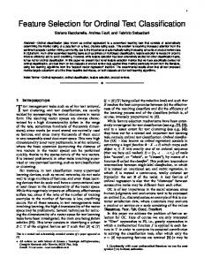
Accuracy of feature selection Fig. 1. Gamma test regression line on the LSU rRNA dataset based on 2-grams, where selected features are included, see Koncar (1997).

the h≤ p nearest neighbours. Both ∆(p) and Γ(p) are easily computed from the data set. As p increases, we might expect to find that Γ(p) grows approximately linearly with ∆(p) for small p. We certainly found this correlation to hold when function f was known to be smooth. The linear correlation of Γ(p) with ∆(p) suggests a possible method for dealing with the fact that in a finite data set we cannot have max |x′ – x| arbitrarily small. We can estimate Γ(p) and ∆(p) for the first several values of p, and extrapolate the regression line to ∆ = 0. The intercept Γ = lim Γ (see Figure 1) will usually give an improved estimate for Var(r). The Gamma test can be used to estimate the best embedding dimension: the minimal Γ corresponding to the more important and informative subset of features. On data sets which are not excessively large and the number of features m is less then 20, the test is sufficiently fast to be run on a complete examination of all possible 2 m – 1 subsets of features. For a larger number of features, we use a genetic algorithm (in the sense of Holland, 1975). Every feature selection Sj , 1≤ j≤ 2 m – 1 is represented by a binary string of length m, where ‘0’ in the ith position means that the ith feature is excluded from current selection and ‘1’ indicates its presence otherwise. The fitness of each member (individual) Sj of the population {S1, …, SK } (K≤ 2 m – 1) is a function of the Γ-value: Fitness(Sj ) = 1/(1 + eΓ(j)/τ), where τ > 0 is a constant which controls the shape of the fitness curve, and Γ(j) is the Γ-value found by running the Gamma test with features selected according to Sj . An initial population of unique random bit strings is generated and the fitness of each is found as above. In each generation, a set number of breeding events take place. Two parents P1 and P2 are randomly selected from the current population: P1 with a probability proportional to its fitness and P2 uniformly from all individuals. These two parents are combined using a one-point crossover operation, by picking

To estimate the accuracy of feature selection, the proposed method was tested on a set of sequences with known feature preferences. Let us consider Markov chains of order 0 where the symbols from the alphabet {A, C, G, U} occur with probabilities pA, pC, pG and pU. It is clear that the probabilities of corresponding bigrams will be pAA = pA · pA, pAC = pA · pC and so on. Suppose that the training set includes two classes of the sequences over the alphabet {A, C, G, U} generated with the probabilities pA = 0.25, pC = 0.25, pG = 0.25, pU = 0.25 and pA = 0.2, pC = 0.2, pG = 0.3, pU = 0.3. In other words, the sequences from the second class have more letters G or U and, correspondingly, more bigrams GU or UG (pGU = pUG = 0.09) than the sequences from the first class (pGU = pUG = 0.0625). Thus, the frequency of bigrams GU or UG might be a good classification feature for these particular classes. We were therefore encouraged to find that the feature selection method proposed herein, when applied to this problem, does indeed select the frequency of bigram UG as the most informative feature. The analysis of the Markov chains of order 0 with other symbol distributions has shown that if there are asymmetries in bigram frequencies then the feature selection obtained by the method discussed here is the same as expected according to the probabilities of bigrams.

Implementation Ribosomal LSU RNA classification To illustrate its possibilities, the method was used for feature selection and LSU rRNA classification according to RDP phylogenetic classes (Maidak et al., 1994). The RDP database was chosen for the following reasons. First, the RDP database is one of the few databases that organize their entries according to phylogenetic relationships with a high level of accuracy. Second, its size is relatively small. Third, classification and annotation of unknown rRNA sequences is now very important as a method of biosphere monitoring.

141

N.A.Chuzhanova, A.J.Jones and S.Margetts

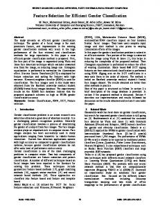
Table 1. LSU rRNA phylogenetic classes Class no.

No. of sequences

Class name

1 2 3 4 5 6 7 8 9 10 11 12

3 11 2 10 23 5 8 2 7 2 9 5

13 14 15 16

6 15 69 4

17 18 19 20

3 21 8 23

Archaea.Crenarchaeota Archaesta:Euryarchaeotata:Archaeoglobales Bacteria:Flavobacteria and relatives Bacteria:Gram Positives and relatives, High G+C Bacteria:Gram Positives and relatives, Low G+C Bacteria:Proteobacteria Alpha Bacteria:Proteobacteria Beta Bacteria:Proteobacteria Epsilon Bacteria:Proteobacteria Gamma Bacteria:Spirochetes Eukarya:Animalia:Arthropoda:Uniramia:Insecta Eukarya:Fungi:Eumycota:Ascomycotina Hemiascomycetes Eukarya:Plantae:Magnoliophyta::Magnoliopsida Eukarya:Protoctista:Zoomastigina::Kinetoplastida Mitochondria:Animalia:Arthropoda:Uniramia:Insecta Mitochoneria:Fungi:Eumycota: Ascomycotina:Plectomycetes Mitochondria:Plantae:Bryophyta::Marchantiopsida Mitochondria:Protoctista:Rhizopoda::Lobosea Plastids:Plantae:Magnoliophyta::Magnoliopsida Plastids:Protoctista:Chlorophyta::Chlorophyceae

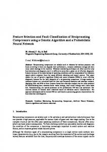
Table 2. Training, embedding and prediction results Group ID

No. of training sequences

No. of selected features f t

1

165

8

2 3 4

160 161 236

10 8 13

Γ value (P≤ 20)

No. of testing sequences

1.92 ×

70

70

84.3

93

75 74 34

74.7 64 80

92 75 91

94.6 88 94

10–7

5.2 × 10–7 2.8 × 10–6 5.1 × 10–9

The data used for the Gamma test contained 236 LSU rRNA from 20 phylogenetic classes (Table 1) derived from the RDP database (Release 5.0, December 13, 1996). Five classes were rejected because each had only one sequence present in the database. The alphabet of RNA includes four symbols {A, C, G, U}. The approximate length of the sequences is 3200–5000 nucleotides. The sequences were represented by their bigram spectrum or, in other words, by 16 features. To make the sequence representation length invariant, all values were scaled by Ni – l + 1 where Ni is the length of the ith sequence. Note that the choice of the length l is very important. Values l = 2, 3 are preferable both from the biological point of view (see the Introduction) and for the robustness of prediction: with l > 3, the training set is separated better but the robustness of prediction falls down (Gusev and Chuzhanova, 1990). To estimate the predictive accuracy of the proposed method, a set of sequences was randomly divided into three

142

Prediction accuracy (%) First fit

5-fits

10-fits

groups of approximately equal size. Two of them were used for feature selection (or training) and one for prediction. All three combinations have been employed. In the fourth case, all 236 LSU rRNA were used for feature selection and 34 other sequences from 10 phylogenetic classes for predicting (i.e. testing). The full embedding has been carried out for each case and subsets of features were selected using the Gamma test. During the prediction phase for each sequence from the test set n nearest neighbours in this selected feature space are computed. The output values of these n nearest-neighbour sequences are then used as outputs for the new sequences. For ‘first fit’ n = 1 and the class number is predicted as simply the class of the first nearest-neighbour sequence. For ‘five fits’ n = 5 and correct classification lies within the set of the first five nearest neighbours, etc. The information about training and testing sets, the number of selected features and prediction results according

Feature selection for genetic sequence classification

to one (first fit), five (5-fits) and 10 nearest neighbours (10-fits) are shown in Table 2. As can be seen from Table 2, the predictive accuracy according to the 10 nearest neighbours is ∼94%. Of course, once the search has been narrowed with high probability to 10 possibilities, then a more detailed examination of these 10 sequences can feasibly complete the classification. For the sequences which are not recognized correctly according to n nearest neighbours, where 1≤ n≤ 10, the predicted n classes, although incorrect, are nevertheless closely located on the phylogenetic tree. It would also be possible to train a neural network using these features and we shall report neural network classification results in a later paper. Here we are more interested in the feature selection procedure.

Conclusions The method of feature selection and classification described here does not require searches for homologies, common subsequences or specific patterns, all of which are very time consuming. It gives the opportunity to classify the new sequences into predefined classes on the phylogenetic tree without sequence alignment. The method is robust in the sense that, when errors occur, the incorrect classification is phylogenetically close to the correct classification. Experiments with neural networks on the 72 LSU rRNA from 15 phylogenetic classes derived from the same database have been reported (Wu, 1996). The sequences were represented by their octagram spectrum (l = 8). The singular value decomposition method was used to reduce the number of octagrams to 40. In comparison, the predictive accuracies are higher, from 92 to 100%. Nevertheless, the results of Gusev and Chuzhanova (1990) suggest that methods based on the frequency of longer l-grams (in fact l > 3) are much less likely to be robust, in the sense that given a particular example of a class one can readily find an extended l-gram whose presence characterizes this example uniquely. However, the same l-gram is relatively unlikely to occur without any mutations in another example of the same class. Thus, frequencies of a diverse range of shorter l-grams taken together are likely to provide a much more robust classification. This is a preliminary account of a new technique and is principally designed to show that the method has promise.

One can envisage many improvements, e.g. the Euclidean metric may not be the most appropriate given the context, and the weighting of features could be continuous rather than discrete, but these are questions that can reasonably be addressed in future studies. Of course, it is also possible to improve the prediction accuracy by enlarging the training set and by increasing the quality of the samples.

References Chuzhanova,N. (1989) Inductive method of program synthesis for symbolic sequence processing. In Lecture Notes in Artificial Intelligence. Springer-Verlag, Berlin, Vol. 397, pp. 317–327. Cowe,E. and Sharp,P.M. (1991) Molecular evolution of bacteriophages: discrete patterns of codon usage in T4 genes are related to the time of gene expression. J. Mol. Evol., 33, 13–22. Friedman,J.H., Bentley,J.L. and Finkel,R.A. (1977) An algorithm for finding best matches in logarithmic expected time. ACM Trans. Math. Software, 3, 200–226. Grantham,R., Gautier,C., Gouy,M., Mercier,R. and Pave,A. (1980) Codon catalog usage and genome hypothesis. Nucleic Acids Res., 8, 49–62. Gusev,V.D. and Chuzhanova,N.A. (1990) The algorithms of recognition of the functional sites in genetic texts. In Proceedings of the First International Workshop on Algorithmic Learning Theory. Japanese Society for Artificial Intelligence, Tokyo, pp. 109–119. Hobohm,U., Houthaeve,T. and Sander,C. (1994) Amino acid analysis and protein database compositional search as a rapid and inexpensive method to identify proteins. Anal. Biochem., 222, 202–209. Holland,J. (1975) Adaptation in Natural and Artificial Systems. MIT Press, Cambridge, MA. Koncar,N. (1997) Optimisation methodologies for direct inverse neurocontrol. PhD Thesis, Department of Computing, Imperial College, London. Maidak,B. et al. (1994) The ribosomal database project. Nucleic Acids Res., 22, 3485–3487. Nussinov,R. (1984) Strong duplet preferences in nucleotide sequences and DNA geometry. J. Mol. Evol., 20, 111–119. Pietrokovski,S., Hirshon,J. and Trifonov,E.N. (1990) Linguistic measure of taxonomic and functional relatedness of nucleotide sequences. J. Biomol. Struct. Dyn., 7, 1251–1268. Stefánsson,A., Koncar,N. and Jones,A.J. (1997) A note on the Gamma test. Neural Comput. Applic., 5, 131–133. Wu,C.H. (1996) Gene classification artificial neural system. Methods Enzymol., 266, 71–88.

143