JMLR: Workshop and Conference Proceedings 10: 76-85 The Fourth Workshop on Feature Selection in Data Mining
Feature Selection for Text Classification Based on Gini Coefficient of Inequality Sanasam Ranbir Singh
[email protected]
Department of Computer Science and Engineering Indian Institute of Technology Guwahati Guwahati 781039, Assam, India
Hema A. Murthy
[email protected]
Department of Computer Science and Engineering Indian Institute of Technology Madras Channai 600036, Tamil Nadu, India.
Timothy A. Gonsalves
[email protected]
Department of Computer Science and Engineering Indian Institute of Technology Madras Channai 600036, Tamil Nadu, India
Editor: Huan Liu, Hiroshi Motoda, Rudy Setiono, and Zheng Zhao
Abstract A number of feature selection mechanisms have been explored in text categorization, among which mutual information, information gain and chi-square are considered most effective. In this paper, we study another method known as within class popularity to deal with feature selection based on the concept Gini coefficient of inequality (a commonly used measure of inequality of income). The proposed measure explores the relative distribution of a feature among different classes. From extensive experiments with four text classifiers over three datasets of different levels of heterogeneity, we observe that the proposed measure outperforms the mutual information, information gain and chi-square static with an average improvement of approximately 28.5%, 19% and 9.2% respectively. Keywords: Text categorization, feature selection, gini coefficient, within class popularity
1. Introduction Text categorization (TC) is a supervised learning problem where the task is to assign a given text document to one or more predefined categories. It is a well-studied problem and still continues to be topical area in information retrieval (IR), because of the ever increasing amount of easily accessible digital documents on the Web, and, the necessity for organised and effective retrieval. High dimensionality of feature space is a major problem in TC. The number of terms (i.e., features) present in a collection of documents, in general, is large and few are informative. Feature selection for TC is the task of reducing dimensionality of feature space by identifying informative features and its primary goals are improving classification effectiveness, computational efficiency, or both. The performance of a classifier is affected by the employed feature selection mechanism. c ⃝2010 Singh, Murthy and Gonsalves.
Feature Selection for Text Classification Based on Gini Coefficient of Inequality
This paper proposes a feature selection mechanism called within class popularity (WCP) which addresses two improtant issues of feature selection for text classification i.e., uneven distribution of prior class probability and global goodness of a feature. The performance of WCP is then compared with the performance of the most commonly used measures – mutual information (MI), information gain(IG), chi-square(CHI). The rest of the paper is organised as follows. Section 2 reviews few related studies. Section 3 presents the proposed feature selection. Section 4 presents experimental evaluations. The paper concludes in Section 5.
2. Review of Few Related Studies At present feature selection methods for TC are based on statistical theory and machine learning. Some well-known methods are information gain, term frequency, mutual information, chi-square statics, Gini index (Yang and Pedersen, 1997; Shankar and Karypis, 2000). We briefly review these measures in this section. 2.1 Mutual Information: P r(t,c) Mutual information (MI) between a term t and a class c is defined by M I(t, c) = log P r(t)P r(c) . To measure the global goodness of a term in feature selection, we combine the category specific scores as M Imax (t) = maxi M I(t, ci ). ∑ Alternatively, in some studies (Yang and Pedersen, 1997), it is also define as M Imax (t) = i P r(ci )M I(t, ci ).
2.2 Information Gain: It is defined by following expression (Yang and Pedersen, 1997). ∑ ∑ IG(t) = − i P r(c ∑ i ) log P r(ci ) + P r(t) i P r(ci |t) log P r(ci |t) +P r(t¯) i P r(ci |t¯) log P r(ci |t¯) It is frequently used as a term goodness criterion in machine learning. It measures the number of bits required for category prediction by knowing the presence or the absence of a term in the document. 2.3 χ2 static: The χ2 static (CHI) is defined by the following expression (Yang and Pedersen, 1997). χ2 (t, c) =
N × (AD − CB)2 (A + C) × (B + D) × (A + B) × (C + D)
where N is the number of documents, A is the number of documents of class c containing the term t, B is the number of documents of other class (not c) containing t, C is the number of documents of class c not containing the term t and D is the number of documents of other class not containing t. It measures the lack of independence between t and c and comparable to χ2 distribution with one degree of freedom. The commonly used global goodness 2 2 estimation ∑ functions2 are maximum and mean functions i.e.,χ (f ) = arg maxci χ (f, ci ) or 2 χ (f ) = i P r(ci )χ (f, ci ). 77
Singh, Murthy and Gonsalves
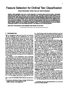
Figure 1: Transformation of samples space.
3. Proposed Feature Selection This section discusses the design and implementation details of the proposed within class popularity (WCP). The implementation details of text classifiers (seed-based, naive Bayes, kNN and SVM) are discussed in the Appendices A. The proposed framework addresses the issues of uneven distribution of prior class probability and global goodness of a feature in two stages. First, it transforms the samples space into a feature specific normalized samples space without compromising the intra-class feature distribution. In the second stage of the framework, it identifies the features that discriminates the classes most by applying gini coefficient of inequality (Lorenz, 1905). 3.1 Transforming Samples Space In the first stage of the proposed framework, we create a normalized samples space for each feature. Given a feature, the goal is to transform the original samples space into a normalized samples space of equal class size without altering the intra-class feature distribution. To transform the samples space, we first define popularity of a feature f within a class by a conditional probability of f given a class label ci i.e. P r(f |ci ) using Laplacian smoothing as follows: 1 + N (f, ci ) ∑ P r(f |ci ) = (1) |V | + f ∈V N (f, ci ) where N (f, ci ) is the number of occurrences of the term f in all the documents in ci and V is the vocabulary set. Such a smoothing is important for classifiers such as naive Bayes where a sequence of the products of conditional probabilities is involved. Other smoothing techniques are also studied in (Wen and Li, 2007). Now, P r(f |ci ) defines intra-class distribution of a feature in a unit space. Thus, for a given feature f , each class can be normalized to the samples size of unit space without compromising feature distribution. Figure 1 shows the transformation pictorially. Dark area represents the portion of the samples containing the feature f in a class. In the normalized samples space, classes are evenly distributed. In an uniform space, the probability P r(ci |f ) (i.e., given a term f , what is the probability that a document belongs to the class ci ) is often effectively used to estimate the confidence weight of an association rule in data mining. We therefore apply the same concept to estimate the association between a 78
Feature Selection for Text Classification Based on Gini Coefficient of Inequality
100% Cumulative share of income (%)
Line of equality
A
B Lorenz curve
100% Cumulative share of population from lowest to highest (%)
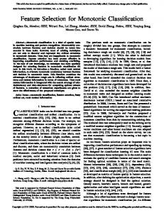
Figure 2: (a) Graphical representation of the Gini index coefficient. class and a feature. We now normalize the above popularity weight (i.e. Equation 1) across all classes and define within class popularity as follows. P r(f |ci ) wcp(f, ci ) = ∑|C| k=1 P r(f |ck )
(2)
where C is the set of the class labels. It has the following characteristics: ∑ • i wcp(f, ci ) = 1. • wcp(f, ci ) ranges between (0, 1) i.e., 0 < wcp(f, ci ) < 1. It is because P r(f |ci ) > 0. • if a term f is evenly distributed across all classes then wcp(f, ci ) = 1/|C|∀ci ∈ C. • if wcp(f, ci ) > wcp(f, cj ), then feature f is present more densely in the class ci than class cj . • if wcp(f, ci ) ≈ 1, then the feature f is likely to be present only in the class ci . Remark 1 The wcp(f, ci ) is equivalent to P r(ci |f ) in the normalized samples space. Since the classes are evenly distributed in the normalized samples space, wcp(f, ci ) is un-biased to prior class probability. As effectively used in association rules mining, with a reasonably high support weight (i.e., P r(f |ci )), a high value of wcp(f, ci ) can represent high association between a class and a feature. A conceptually similar feature selector has been used in (Aggarwal et al., 2004). However the estimator does not use smoothing while calculating P r(f |ci ). Another difference is that it uses the square root of the sum of squares to estimate the distribution of a feature across different classes, whereas we use gini coefficient of inequality. 3.2 Global Goodeness of a term Commonly used global goodness estimators are maximum and average functions. Our goal is to identify the features that discriminates the classes most. A good discriminant term will 79
Singh, Murthy and Gonsalves
have skewed distribution across the classes. However, these two functions do not capture how a feature is distributed over different classes. We use gini coefficient of inequality, a popular mechanism to estimate the distribution of income over a population, to analyse distribution of a feature across the classes. Pictorially, it can be shown as the plots in Figure 2. In the figure, gini of a population is defined by the area marked “A” divided by the areas marked “A” and “B” i.e., gini = A/(A + B). If gini = 0, every person in the population receives equal percentage of income and if gini = 1, single person receives 100% of the income. A commonly used approach to represent the inequality and estimate the area under the curve is Lorenz Curve (Lorenz, 1905). In Lorenz curve, individuals are sorted by size in increasing order and the cumulative proportion of individuals (x-axis) is plotted against the corresponding cumulative proportion of their total size on y-axis. If we have a sample of n classes, then the sample Lorenz curve of a term t ∑ is the polygon joining the points (h/n,Lh /Ln ), where h = 0, 1, 2, 3..., n, L0 = 0 and Lh = hi f (t, ci ) (Kotz et al., 1983). As shown in (Dixon et al., 1987), if the data is ordered increasing size, the Gini coefficient is estimated as follows. ∑n (2i − n − 1)wcp(t, ci ) (3) G(t) = i=1 n2 µ where µ is sample mean. It has been shown that sample Gini coefficient calculated by Equation (3) is biased and is to be multiplied by n/(n − 1) to become unbiased. 3.3 Performance Metric We use F1 measure (VanRijsbergen, 1979) to present performance of a classifier. F-measure is computed by calculating the harmonic mean of precision and recall as follows: F =
α.P recision.Recall P recision + Recall
F1-measure is commonly used F-measure where α = 2. Precision is the ratio of correctly classified documents to the number of classified documents and recall is the ratio of correctly classified documents to the number of test documents. The F-measure is a binary class performance metric. In order to estimate F1-value for multi-class problem, we have used micro-average estimation (Yang, 1999).
4. Experimental Results The performance of feature selection mechanisms are evaluated using four classifiers – seedbased, naive Bayes, kNN and SVM (Appendix A) over three datasets – Reuters-21578, 7Sectors-WebKB and a scan of the Open Directory Project. The classification performances over these datasets are evaluated using 5-fold cross validation: four fold for training and one fold for testing and average over the 5-folds. 4.1 Datasets and Characteristics Table 1 summerizes the characteristics of the datasets. We briefly discuss the three datasets as follows: 80
Feature Selection for Text Classification Based on Gini Coefficient of Inequality
Table 1: Characteristics of the Datasets. ‡ average over 5-fold after performing Porter stemming (Porter, 1980) and ignoring stopwords Datasets
Reuters
ODP
7-Sectors
21578
4,19,725
4582
13,918.6
16,49,152
24,569.2
3,845.4
28,721.6
6,288
63.8
346.4
194.8
38.1
131.9
96.5
10
17
7
Evaluation Methodology
5-fold
5-fold
5-fold
Number of examples per fold
1,593
83,945
916
Number of Documents Number of
Terms‡
Number of Terms selected‡ . Average Document size Average #unique words/doc Number of Categories
• Reuters-21578 It is a highly skewed dataset containing 21578 news articles. For our experiments, we consider documents which are marked with TOPICS label. To ensure that each category contains a good number of training documents, as done in (Wang et al., 2007), we have considered the top 10 largest categories. We have considered the terms whose document frequency is at least 5. • 7-Sectors WebKB It is slightly skewed. We have considered the terms whose document frequency is at least 5. These documents are collected from different Web sources, which are developed and maintained by different groups of people. • Open Directory Project We use Open Directory Project taxonomy from the March 2008 archive. This taxonomy consists of 4,592,207 number of urls and 17 classes in its top label. We have arbitrarily selected 419725 number of urls and locally crawled. We have considered the terms whose document frequency is at least 100. 4.2 Performance of Feature Selection Mechanisms The experiments are executed with different feature space. Initially, features are ordered by their global goodness weights and then define the feature dimension by 10%, 20% and so on up to 100% of the selected features (refer Table 1). Table 2 shows a comparison of microaverage F1 measures among feature selectors using four text classifiers (seed-based, naive Bayes, kNN and SVM). It shows the minimum, average and maximum micro-average F1 values of different classifiers over different feature dimensions with different feature selectors over different datasets. All four classifiers perform relatively well using WCP. Except on two instances i.e., Naive Bayes with CHI over Reuters-21578 and 7Sectors-WebKB datasets, WCP outperforms all other feature selectors in all instances. It is also observed that all four text classifiers perform relatively well on news dataset (Reuters-21578). The performance of the classifiers over 7Section-WebKb is moderate and performance over Open Directory Project is poor. 81
Singh, Murthy and Gonsalves
Table 2: Show minimum, average and maximum value of micro average F1 measure across different classifiers using different feature selectors Reuters-21578 Collections FS
Seed
kNN
SVM
NB
Min
Avg
Max
Min
Avg
Max
Min
Avg
Max
Min
Avg
Max
WCP
0.91
0.94
0.95
0.91
0.92
0.94
0.89
0.91
0.93
0.90
0.94
0.96
CHI
0.81
0.81
0.81
0.90
0.91
0.92
0.83
0.89
0.90
0.93
0.947
0.95
IG
-
-
-
0.83
0.85
0.86
0.84
0.88
0.89
0.86
0.89
0.90
MI
0.26
0.58
0.86
0.49
0.78
0.91
0.56
0.77
0.89
0.27
0.59
0.90
Open Directory Project Collections FS
Seed
kNN
SVM
NB
Min
Avg
Max
Min
Avg
Max
Min
Avg
Max
Min
Avg
Max
WCP
0.21
0.46
0.55
0.25
0.44
0.52
0.38
0.48
0.56
0.22
0.45
0.54
CHI
0.20
0.38
0.45
0.21
0.40
0.49
0.36
0.41
0.46
0.21
0.42
0.50
IG
-
-
-
0.19
0.38
0.47
0.31
0.32
0.33
0.32
0.33
0.37
MI
0.36
0.43
0.45
0.15
0.25
0.35
0.19
0.28
0.32
0.26
0.39
0.46
7-Sectors-WebKB Collections FS
Seed
kNN
SVM
NB
Min
Avg
Max
Min
Avg
Max
Min
Avg
Max
Min
Avg
Max
WCP
0.55
0.64
0.67
0.45
0.52
0.56
0.45
0.54
0.57
0.51
0.61
0.66
CHI
0.53
0.61
0.61
0.35
0.42
0.45
0.41
0.43
0.48
0.55
0.62
0.72
IG
-
-
-
0.43
0.50
0.52
0.39
0.42
0.44
0.43
0.46
0.48
MI
0.39
0.55
0.59
0.45
0.50
0.53
0.35
0.44
0.47
0.38
0.55
0.63
It verifies the claim that traditional text classifiers with traditional feature selectors are not suitable for extremely heterogeneous dataset. Table 3 shows the average performance of each feature selector across all classifiers and datasets. Table 4 shows the performance improvement of different classifiers when they use WCP feature selector over the performance obtained by the same classifier using MI, CHI and IG feature selectors. There is an overall improvement of 25.4% over MI, 6.8% over CHI, and 16.2% over IG. In brief, we have observed the following – (i) Overall WCP is suitable for all datasets, (ii) Overall WCP is suitable for all classifiers, (iii) MI performs the least among the feature selectors, (iv) all four classifiers perform equally well on Reuters-21578 dataset, (v) With carefully selected examples (7Sectors-WebKB), traditional text classifiers can also provide high performance on Web document collections. 82
Feature Selection for Text Classification Based on Gini Coefficient of Inequality
Table 3: Average performance over all classifiers using different datasets and over all datasets using different classifier Over all Classifiers Feature Selector
Over all datasets
Reuters
Sectors
ODP
Seed
kNN
SVM
NB
Within-Class-Popularity
0.93
0.58
0.46
0.68
0.63
0.64
0.67
CHI-square
0.89
0.52
0.4
0.6
0.577
0.577
0.663
Information Gain
0.876
0.46
0.34
-
0.577
0.54
0.56
Mutual Information
0.68
0.51
0.34
0.52
0.51
0.497
0.51
Table 4: Improvement in performance of different classifiers using WCP over other feature selectors Seed
kNN
NB
SVM
Reuters
7Sectors
ODP
Overall
13.2%
8.6%
1.5%
10.3%
4.5%
11.5%
15%
9.2%
Over IG
-
8.6%
18.5%
19.6%
5.7%
26.1%
35.3%
19%
Over MI
30.5%
23.5%
28%
31.4%
36.8%
13.7%
35.3%
28.5%
Over CHI
5. Conclusion In this paper we study a feature selection mechanism called within-class-popularity, which measures normalized popularity of a term within a class. It uses Gini coefficient of inequality to estimate global goodness of a term. The performance of WCP is then compared with that of mutual information, chi-square and information gain using four text classifiers (seedbased, kNN, naive Bayes and SVM) over three datasets (Reuters-21578, 7Sectors-WebKB and Open Directory Project). From extensive experiments, it is found that on an average WCP outperforms MI, CHI and IG feature selectors.
References C. C. Aggarwal, S. C. Gates, and P. S. Yu. On using partial supervision for text categorization. IEEE Transaction. on Knowledge and Data Engineering, 16 (2):245–255, 2004. P. M. Dixon, J. Weiner, T. Mitchell-Olds, and R. Woodley. Bootstrapping the gini coefficient of inequality. Ecology, 65 (5):1548–1551, 1987. S. Kotz, N. L. Johnson, and C. B. Read, editors. Encyclopedia of statistical science. John Wiley and Sons, NY, USA, 1983. M. O. Lorenz. Methods of measuring the concentration of wealth. American Statistical Association, 9 (70):209–219, 1905. 83
Singh, Murthy and Gonsalves
M.F. Porter. An algorithm for suffix stripping. Program: electronic library and information systems, 14 (3):130–137, 1980. G. Salton, A. Wong, and C. S. Yang. A vector space model for automatic indexing. ACM Communication, 18 (11):613–620, 1975. S. Shankar and G. Karypis. Weight adjustment schemes for a centroid based classifier. Technical Report TR00-035, University of Minnesota, 2000. C. VanRijsbergen. Information Retrieval. Butterworths, London, 1979. Z. Wang, Q. Zhang, and D. Zhang. A pso-based web document classification algorithm. In Proc. the Eighth ACIS International Conference on Software Engineering, Artificial Intelligence, Networking, and Parallel/Distributed Computing (SNPD 2007), pages 659– 664, 2007. J. Wen and Z. Li. Semantic smoothing the multinomial naive bayes for biomedical literature classification. In Proc. of the 2007 IEEE International Conference on Granular Computing (GRC ’07), 2007. Y. Yang. An evaluation of statistical approaches to text categorization. Information Retrieval, 1 (1-2):69–90, 1999. Y. Yang and J. O. Pedersen. A comparative study on feature selection in text categorization. In Proc. the Fourteenth International Conference on Machine Learning (ICML-97), pages 412–420, 1997.
Appendix A. Experimental Text Classifiers We use vector space model to represent documents (Salton et al., 1975) for the TC. In vector space model, a document d is represented by a term vector of the form d = {w1 , w2 , ..., wn }, where wi is a weight associated with the term fi . We use TF-IDF and cosine normalisation (Aggarwal et al., 2004) to define the weight of a feature fi in a document vector d as follows; wi = √∑tfn idf (fi ,d) 2 and tf idf (fi , d) = tf (fi , d). log dfD|D| (fi ) , where tf (fi , d) is the k
tf idf (fk ,d)
term frequency of fi in d, D is the document set and dfD (fi ) is document frequency of the term fi . A.1 Seed-based Classifier In our study, we design a Seed-based classifier (also known as centroid based classifier) especially for WCP. Each class is represented by a term vector known as seed. We define a pseudo-seed ci for each class ci as follows: ci = {wf |wf = wcp(f, ci ), ∀f ∈ F }
(4)
where F is a set of selected features. Given a test example d defined over F , we classify d by the following function.classif y(d) = arg maxci {cosine(d, ci )} where cosine(d, ci ) is the cosine similarity between d and ci . IG does not provide class specific weight. Therefore, it is omitted from exploring the seed-based classifier. 84
Feature Selection for Text Classification Based on Gini Coefficient of Inequality
A.2 naive Bayes Assuming naives condition i.e., features are conditionally independent, we defined naive Bayes classifier by ∏ P r(ck ). j P r(dij |ck ) ∏ P r(ck |di ) = j P r(dij ) ∏ As denominator is independent of class, effectively, we have estimated P r(ck |di ) as j P r(dij |ck ), where P r(dij |ck ) is defined by Equation 1 A.3 kNN Cosine similarity is used to estimate distance between test examples and training examples. For each test sample, at most 30 nearest neighbours are considered to count for the winner class. In the case of Open Directory Project dataset having very large number of documents, we have randomly selected only 100 test examples from each class and 400 examples from each training class and estimated similarity between 1700 test examples and 6800 training examples. A.4 SVM We use the SVMTorch software 1 for our reported estimations, which is publicly available for download. Again training SVM with large dataset is very expensive. Therefore, like kNN, we have randomly selected only 100 test examples and 400 training examples from each class. We run svm tool using linear kernel. From various experiments, we find that linear kernel perform better compared to radial and Gaussian kernel.
1. SVMTorch: an SVM software for Classification and Regression, in C++,http://www.idiap.ch/ machine-learning.php
85