Feature Selection in Proteomic Pattern Data with Support Vector Machines Kees Jong∗, Elena Marchiori∗ , Mich`ele Sebag† , Aad van der Vaart∗ ∗ Department
of Mathematics and Computer Science Vrije Universiteit Amsterdam, The Netherlands Email: cjong,elena,
[email protected] † Laboratoire de Recherche en Informatique, CNRS UMR 8623 Universit Paris-Sud Orsay, France Email:
[email protected]
Abstract— This paper introduces novel methods for feature selection (FS) based on support vector machines (SVM). The methods combine feature subsets produced by a variant of SVM-RFE, a popular feature ranking/selection algorithm based on SVM. Two combination strategies are proposed: union of features occurring frequently, and ensemble of classifiers built on single feature subsets. The resulting methods are applied to pattern proteomic data for tumor diagnostics. Results of experiments on three proteomic pattern datasets indicate that combining feature subsets affects positively the prediction accuracy of both SVM and SVM-RFE. A discussion about the biological interpretation of selected features is provided.
I. I NTRODUCTION FS can be formalized as a combinatorial optimization problem, finding the feature set maximizing the quality of the hypothesis learned from these features. FS is viewed as a major bottleneck of supervised learning and data mining [1], [2]. For the sake of the learning performance, it is highly desirable to discard irrelevant features prior to learning, especially when the number of available features significantly outnumbers the number of examples, as is the case in bioinformatics. In particular, biological experiments from laboratory technologies like microarray and proteomic techniques, generate data with very high number of attributes, in general much larger than the number of examples. Therefore FS provides a fundamental step in the analysis of such type of data [3]. By selecting only a subset of attributes, the prediction accuracy can possibly improve and more insight in the nature of the prediction problem can be gained. A number of effective FS methods for classification rank features and discard those whose rank is smaller than a given threshold [1], [4]. This threshold can be either provided by the user, like in [5], or automatically determined, like in [6], by means of the estimated rank of a new random feature. A popular algorithm based on the above approach is SVMRFE [5]. It is an iterative algorithm. Each iteration consists of the following two steps. First feature weights, obtained by training a linear SVM on the training set, are used in a scoring
function for ranking features. Next, the feature with minimum rank is removed from the data. In this way, a chain of feature subsets of decreasing size is obtained. SVM classifiers are trained on training sets restricted to the feature subsets, and the classifier with best predictive performance is selected. In the original SVM-RFE algorithm one feature is discarded at each iteration. Other choices are suggested in [5], where at each iteration features with rank lower than a user-given theshold are removed. The choice of the threshold affects the results of SVM-RFE. Heuristics for choosing a threshold value have been proposed [5], [6]. In this paper the problem of choosing a threshold is sidestepped by considering multiple runs of SVM-RFE with different thresholds. Each run produces one feature subset. The resulting feature subsets are combined in order to obtain a robust result/classification. Two methods for building a classifier from a combination of feature subsets are proposed, called JOIN and ENSEMBLE. JOIN generates a classifier by training SVM on data restricted to those features that occur more than a given number of times in the list of feature subsets. ENSEMBLE generates a majority vote ensemble of classifiers, where each classifier is obtained by training SVM on data restricted to one feature subset. This combination strategy is used, e.g., in [7], where decision trees trained on data restricted to randomly selected feature subsets are ensembled. JOIN and ENSEMBLE are compared experimentally with SVM trained on all features, and with a multistart version of SVM-RFE. Multistart SVM-RFE performs multiple runs of SVM-RFE with different thresholds, and selects among the resulting feature subsets the one minimizing the error (on hold-out set) of SVM trained on data restricted to that feature subset. The four methods are applied to pattern proteomic data from cancer and healthy patients. This type of data is used for cancer detection and potential biomarker identification. Motivations for choosing FS methods based on linear SVM are their robustness with respect to high dimension input data, and the experimental observation that such data appear to be almost linearly separable (see e.g., [8], [9]).
Experiments are conducted on three pattern proteomic data from prostate and ovarian cancer. On two of the three datasets JOIN and ENSEMBLE achieve significantly better predictive accuracy than SVM and multistart SVM-RFE. On the third dataset JOIN obtains perfect classification and the other methods almost perfect classification. The results indicate that FS methods combining feature subsets from multiple runs provide a robust and effective approach for feature selection in proteomic pattern data. The paper is organized as follows. Section II gives an overview of the considered FS methodology. Section III describes the data used in the experiments. Section IV reports on results of the experiments. The paper ends with a discussion and points to future research. II. M ETHODS In linear SVM (binary) classification [10], [11] patterns of two classes are linearly separated by means of a maximum margin hyperplane, that is, the hyperplane that maximizes the sum of the distances between the hyperplane and its closest points of each of the two classes (the margin). When the classes are not linearly separable, a variant of SVM, called soft-margin SVM, is used. This SVM variant penalizes misclassification errors and employs a parameter (the soft-margin constant C) to control the cost of misclassification. When the two classes are unbalanced, different penalty for misclassification can be associated to each class. This can be realized in SVM by means of two C parameters, Cc = C ∗ wc (for cancer class patterns) and Ch = C ∗wh (for healthy ones). Training a linear SVM classifier produces a decision function of the form f (x1 , . . . , xN ) =
N X
w i xi + b
i=1
The weights wi provide information about feature relevance, where bigger weight size implies higher feature relevance. In this paper feature xi is scored by means of the absolute value of wi . Other scoring functions based on weight features are possible, like, e.g., wi2 , which is used in the original SVM-RFE algorithm [5]. In order to perform feature selection and to assess the method, the dataset is partitioned in three subsets: a train set (T), a hold-out set (H) and a validation set (V). The sets T, H are used for generating a classifier and V is used for assessing its predictive performance on unseen examples. Linear SVM is used in the popular feature ranking method SVM-RFE, which starts with all features and generates a ranking by removing at each iteration a feature with worst weight score. The following FS method based on SVM-RFE is introduced. SVM-RFE(threshold) begin
i :=0; F_i := {all input features} while (F_i not empty) Train linear SVM on T restricted to F_i Rank the features of F_i F_i+1 := F_i - {threshold percent of features in F_i with smallest rank} i := i+1; end F* := F in {F_0,...,F_i-1} such that SVM_|F has minimum error on H restricted to F output = SVM_|F* end SVM-RFE(threshold) discards at each iteration a percentage (specified by the parameter threshold) of the actual number of features. The algorithm generates a chain of feature subsets of decreasing size, one set at each iteration. Each subset is evaluated using the following scoring function: score(F ) = err(SV M|F ) + |F |/N, where err(SV M|F ) is the error on H of SVM trained on T restricted to F , |F | denotes the size of F , and N the total number of features. The second term of the sum penalizes large feature subsets. A feature subset F ∗ having minimum score is selected, and SVM trained on T restricted to F ∗ , denoted by SVM |F*, is returned as output. The two methods proposed in the sequel combine feature subsets obtained by multiple runs of SVM-RFE(threshold) using different threshold values. The following pseudo-code describes the two algorithms, called JOIN and ENSEMBLE. JOIN(cutoff,v1,...,vk) begin for theshold v in {v1, ..., vk} F(v) = SVM-RFE(v) end F* := features occurring at least cutoff times in (F(v1), ..., F(vk)) output = SVM_|F* end ENSEMBLE(v1,...,vk) begin for threshold v in {v1, ..., vk} F(v) = SVM-RFE(v) end output = majority vote classifier using SVM_|F(v1), ... , SVM_|F(vk) end JOIN(cutoff,v1,...,vk) constructs one set of features from feature subsets obtained by running SVM-RFE(threshold) with threshold value in v1,...,vk. Features occurring at least cutoff
time in the resulting list of feature subsets are selected and SVM is trained on T restricted to those features.
such that the graph should be considered a smoothed version of the true mass density.
ENSEMBLE(v1,...,vk) generates a list of feature subsets by applying SVM-RFE(threshold) with threshold value in v1,...,vk. Each resulting feature subset F is used to train one SVM classifier on T restricted to F. The algorithm ensembles the trained SVM classifiers using the majority vote as classification criterion.
Given proteomic profiles for a sample of healthy and diseased individuals it is desired to build a classifier for tumor diagnostics and to identify the protein masses that are potentially involved in the disease. Because of the large number of features (the m/z ratios) and the small sample size (the specimens), these two problems are tackled using heuristic algorithms for feature selection.
EXAMPLE IV. E XPERIMENTS The following toy example illustrates the application of JOIN and ENSEMBLE. Suppose a dataset with patterns consisting of four features, say 1,2,3,4, is given. Suppose the user considers three threshold values, say 0.1, 0.2, 0.3, and cutoff value 3. SVM-RFE(0.i) generates feature subset F i, for i ∈ [1, 3]. Suppose F 1={1, 3}, F 2={1, 2, 3}, F 3={1, 3, 4}. ENSEMBLE(0.1,0.2,0.3) outputs classifier SV M |{1, 3} ∪ SV M |{1, 2, 3} ∪ SV M |{1, 3, 4}, the ensemble classifier with majority vote consisting of the three SVM classifiers trained on T restricted to feature subsets {1, 3}, {1, 2, 3}, and {1, 3, 4}, respectively. Only features 1 and 3 occur at least 3 times in (F 1, F 2, F 3). Then JOIN(3,0.1,0.2,0.3) produces classifier SV M |{1, 3}, the SVM classifier trained on T restricted to feature subset {1, 3}.
The following experimental setup is used. T, H, and V contain 50, 25, and 25 % of the data, respectively. The following experiments are performed. 1) Train SVM on T∪H using all features. 2) Run SVM-RFE(threshold) with threshold in {0.2, 0.3, 0.4, 0.5, 0.6, 0.7}. 3) Run JOIN(cutoff, 0.2, 0.3, 0.4, 0.5, 0.6, 0.7), with cutoff value in {1, 2, 3, 4, 5} and select the result with best sensitivity on H. 4) Run ENSEMBLE(0.2, 0.3, 0.4, 0.5, 0.6, 0.7). Ten random partitions of the dataset in T,H,V are generated. Performance is measured by means of average, over ten V’s, sensitivity (number of cancer samples correctly classified divided by total number of cancer samples) and specificity (number of healthy samples correctly classified divided by total number of healthy samples). The implementation of the methods uses the LIBSVM library for SVM by Chang and Lin.
III. P ROTEOMIC PATTERN DATA Three proteomic pattern datasets from prostate and ovarian cancer are considered. The datasets are publically available from the NCI/CCR and FDA/CBER Clinical Proteomics Program Databank1. This type of data is obtained by surfaceenhanced laser desorption/ionization time-of-flight mass spectronomy (SELDI-TOF MS), a recent laboratory technology which offers high-throughput protein profiling. It measures the concentration of low molecular weight peptides in complex mixtures, like serum (cf. e.g. [12]). Because it is relatively inexpensive and noninvasive, it is a promising new technology for classifying disease status. SELDI-TOF MS technology produces a graph of the relative abundance of ionized peptides (y-axis) versus their mass-tocharge (m/z) ratios (x-axis). (Cf. Figure 1) The m/z ratios are proportional to the peptide masses, but the technique is not able to identify individual peptides, because different peptides may have the same mass and because of limitations in the m/z resolution. Currently the graph is represented by about 15000 measuring points. There is no obvious relation between neighbour measurement points, apart from the fact that they refer to peptides of similar masses and that the resolution is 1 see
http://clinicalproteomics.steem.com/
A. Prostate Dataset This dataset consists of 322 patterns, containing measurements from 69 cancer patients and 253 healthy (or with a benign disease) persons. Each pattern consists of 15154 features (m/z values). The sizes of T,H and V are 162, 80 and 80, respectively. The following values are used in all experiments: C = 1, wc = 1000, wh = 0.005. These values have been chosen after conducting few experiments on one training set. No exhaustive cross validation for selecting these values has been performed. Observe that a much higher misclassification penalty is assigned to cancer patterns in order to bias the classifier to diagnose correctly (early) cancer patients. It is interesting to investigate whether results of SVM-RFE depend on the choice of the threshold. Table I shows, for each dataset partition, threshold number t and performance of the SVM-RFE(0.t) achieving best sensitivity on V. The results indicate that the threshold value yielding best sensitivity depends on the partition. Figure 2 plots average sensitivity and specificity over the 10 V’s versus threshold values. Sensitivity seems to improve when bigger thresholds are used till the threshold value
100
90
80
70
intensity
60
50
40
30
20
10
0
0
0.2
0.4
Fig. 1.
SENSITIVITY 0.9412 1.0000 0.8235 1.0000 0.8824 0.8824 1.0000 1.0000 0.9412 0.8235
0.6
0.8
1 m/z values
1.2
1.4
1.6
1.8
2 4
x 10
A protein profile generated by SELDI-TOF MS of a patient with ovarian cancer.
SPECIFICITY 0.8889 0.9206 0.9524 0.8571 0.8730 0.9683 0.9206 0.9683 0.9206 0.8730
THRESHOLD NR 5 3 6 3 2 6 4 4 2 4
0.96 sensitivity specificity 0.94
0.92
0.9
0.88
0.86
TABLE I P ROSTATE DATASET. E ACH ROW CONTAINS THE FOLLOWING RESULTS ON ONE DATASET PARTITION : SENSITIVITY, SPECIFICITY FOR THE THRESHOLD NUMBER ( THIRD COLUMN ) ACHIEVING BEST SENSITIVITY
( ON THE
VALIDATION SET ).
PARTITIONS IS
AVERAGE SENSITIVITY OVER
THE
10
0.84
0.82 0.2
0.25
0.3
0.35
0.4
0.45 0.5 theshold value
0.55
0.6
0.65
0.7
0.9294 ( VARIANCE IS 0.0052), AVERAGE SPECIFICITY IS 0.9143 ( VARIANCE IS 0.0016).
Fig. 2. Prostate dataset. SVM-RFE average sensitivity and specificity versus threshold.
becomes too big causing a drastic decrease in sensitivity. Specificity does not show a clear trend related to threshold.
In summary, on this dataset JOIN and ENSEMBLE have the beneficial effect of improving the capability of the baseline SVM classifier to detect cancer patterns at the price of increasing the number of misclassified healthy patterns.
Results of experiments with the four methods are reported in Table II. SVM alone achieves best specificity, while sensitivity improves when FS methods are used, with best sensitivity obtained by JOIN and ENSEMBLE. Means of the results are compared using the Student’s paired t-test. Mean sensitivity of both JOIN and ENSEMBLE are significantly better than those of SVM-RFE and SVM. No significant difference is obtained when results of SVMRFE and SVM are compared with those of Table I. This shows that JOIN and ENSEMBLE achieve performance comparable to SVM-RFE equipped with an oracle able to choose the threshold yielding best sensitivity on future examples (examples in V).
To the best of our knowledge, the results here obtained on this dataset are the best so far reported in the literature. However, one has to consider that a fair comparison is not possible, due to the different experimental setups used in different works. In the first paper that analyzed this dataset, [13], the authors used only one data partition in train and test set, and obtained 0.95 sensitivity and 0 .78 specificity. They use a FS method based on genetic algorithms that optimizes the class label coherence of the clustering obtained using a self-organizing method. In [8], a wrapper FS method based on genetic algorithms is introduced, which uses SVM as baseline classifier. The algorithm achieves average sensitivity equal to 0.63 and 0.95
METHOD
AVG SENSITIVITY
AVG SPECIFICITY
SVM
0.7824 (0.0062)
0.9698 (0.0011)
SVM-RFE
0.8471 (0.0094)
0.9270 (0.0028)
JOIN
0.9647 (0.0009)
0.9016 (0.0022)
ENSEMBLE
0.9529 (0.0029)
0.8905 (0.0055)
SENSITIVITY 0.9200 1.0000 0.9600 1.0000 0.9200 0.9200 1.0000 0.9200 0.9200 0.9200
TABLE II
SPECIFICITY 0.8929 0.8929 0.8571 0.8929 0.8929 1.0000 0.9286 1.0000 0.9643 0.9643
P ROSTATE D ATASET. AVERAGE SENSITIVITY AND SPECIFICITY ( WITH VARIANCE BETWEEN BRACKETS ) OVER THE
10 VALIDATION SETS .
THRESHOLD NR 3 4 2 3 2 3 2 4 2 4
TABLE III OVARIAN DATASET (4-03-02). E ACH ROW CONTAINS THE FOLLOWING RESULTS ON ONE DATASET PARTITION : SENSITIVITY, SPECIFICITY FOR THE THRESHOLD NUMBER ( THIRD COLUMN ) ACHIEVING BEST
specificity. The algorithm searches for small feature subsets of maximum size equal to 20. Figure 6 shows location and frequency of the features selected by SVM-RFE(t), t in {0.2, 0.3, 0.4, 0.5, 0.6, 0.7} on the 10 T’s. SVM-RFE selected a total of 1430 features, which have been used in JOIN and ENSEMBLE. The corresponding m/z values appear to be located in few segments of neighbour m/z values.
SENSITIVITY ( ON THE VALIDATION SET ). THE
10
PARTITIONS IS
AVERAGE SENSITIVITY OVER
0.9480 ( VARIANCE IS 0.0014 ), AVERAGE
SPECIFICITY IS
0.9286 ( VARIANCE IS 0.0026)
0.945 sensitivity specificity
0.94
B. Ovarian Datasets We consider two ovarian datasets. The following SVM parameter values are used for all experiments: C = 10, wc = 10, wh = 0.5. Class misclassification penalties smaller than those used for the prostate dataset are chosen because these datasets are not as skewed as the prostate one.
0.935
0.93
0.925
0.92
1) Dataset (4-03-02): The ovarian dataset (date 4-03-02) consists of 215 samples, with 100 healthy, 15 benign and 100 cancer patterns. Each pattern consists of 15154 features (m/z values). This dataset was generated by repeating the study of [14] using a different type of chip, the WCX2 chip. Samples were processed by hand and the baseline was subtracted, thus possibly creating negative intensities. T,H and V contain 108, 54 and 53 patterns, respectively. Results reported in Table III indicate that on this dataset the threshold yielding best sensitivity on Vdepends on the data split. Figure 3 plots average sensitivity and specificity over the 10 validation sets versus threshold values. Both average sensitivity and specificity show irregular trend, with a peak of specificity for threshold 0.6, which corresponds to a drop of sensitivity. Table IV contains results of experiments. On this dataset, all methods achieve similar sensitivity, and significantly better specificity of JOIN (p=0.005) and ENSEMBLE (p=0.01) over SVM-RFE. Figure 7 shows the plot of m/z values versus number of occurrences of features selected over all the runs. SVM-RFE selected a total of 991 features, which have been used in JOIN and ENSEMBLE. This dataset was first analyzed by means of the commercial
0.915 0.2
0.25
0.3
0.35
0.4
0.45 0.5 theshold value
0.55
0.6
0.65
0.7
Fig. 3. Ovarian dataset (4-03-02). SVM-RFE average sensitivity and specificity versus threshold.
package PROTEOME QUEST, which integrates ideas of [13] in a software package. Perfect sensitivity and 0.97 specificity was reported. Perfect predictive accuracy is reported in [15]. This method first applies a standardization and smoothing to each data pattern, next ranks features using a univariate FS method and selects a threshold by means of random field theory. The resulting features are incrementally added to a 5-NN classifier and the features yielding best possible classification are selected. The better performance of [15] and [13] is possibly due to the non-linear classifiers used in the methods. 2) Dataset (8-07-02): The ovarian dataset (date 8-07-02) consists of 253 samples, with 91 control and 162 ovarian cancer including early stage cancer samples. This dataset is the most recent of the two ovarian datasets. The chips were prepared using robotic instrument. The baseline was not subtracted. Each pattern consists of 15152 features (m/z values). The train,
METHOD
AVG SENSITIVITY
AVG SPECIFICITY
SVM
0.9280 (0.0028)
0.9500 (0.0020)
SVM-RFE
0.9200 ( 0.0018)
0.9250 ( 0.0032)
JOIN
0.9200 ( 0.0018)
0.9679 (0.001)
ENSEMBLE
0.9200 ( 0.0011)
0.9750 (0.001)
1.005 sensitivity specificity
1
0.995
0.99
TABLE IV OVARIAN DATASET (4-03-02). AVERAGE SENSITIVITY AND SPECIFICITY ( WITH VARIANCE BETWEEN BRACKETS ) OVER
THE
0.985
10 VALIDATION SETS . 0.98
0.975 0.2
hold-out and validation set contains 127, 54 and 62 patterns, respectively. The results reported in Tables V, VI indicate that the two classes of this dataset can be linearly separated. Threshold 0.2 can be used on each data splitting, achieving perfect sensitivity. SENSITIVITY 1.0000 1.0000 1.0000 1.0000 1.0000 1.0000 1.0000 1.0000 1.0000 1.0000
SPECIFICITY 1.0000 0.9545 1.0000 1.0000 1.0000 0.9545 0.9545 1.0000 1.0000 1.0000
THRESHOLD NR 2 2 2 2 2 2 2 2 2 2
TABLE V OVARIAN DATASET (8-07-02). E ACH ROW CONTAINS THE FOLLOWING RESULTS ON ONE DATASET PARTITION : SENSITIVITY, SPECIFICITY FOR THE THRESHOLD NUMBER ( THIRD COLUMN ) ACHIEVING BEST SENSITIVITY ( ON THE VALIDATION SET ).
METHOD
AVG SENSITIVITY
AVG SPECIFICITY
SVM
1 (0)
0.9955 (0.0002)
SVM-RFE
1 (0)
0.9864 (0.0005)
JOIN
1 (0)
1 (0)
ENSEMBLE
1 (0)
0.9909 (0.0004)
0.25
0.3
0.35
0.4
0.45 0.5 theshold value
0.55
0.6
0.65
0.7
Fig. 4. Ovarian dataset (8-07-02). SVM-RFE average sensitivity and specificity versus threshold.
methods have perfect or almost perfect predictive accuracy. However, JOIN is the most robust method, yielding perfect classification over all data partitions. Figure 8 shows location and frequency of features selected by SVM-RFE. SVM-RFE selected a total of 187 features, which have been used in JOIN and ENSEMBLE. The corresponding m/z values appear mostly located in the segment [0,1000]. This dataset was first analyzed using PROTEOME QUEST and then in a number of other works, e.g., [8], [9], [15]–[17], using different feature selection methods. As expected, on this dataset all methods obtained perfect or almost perfect predictive performance. SVM-RFE applied to the two ovarian datasets selects a number of common m/z values in the intervals [0,1000], around 4000, 8000 and 9000. However, the ovarian (4-03-02) dataset is not linearly separable and SVM seems to require more features in order to obtain good performance. V. D ISCUSSION
TABLE VI OVARIAN DATASET (8-07-02). AVERAGE SENSITIVITY AND SPECIFICITY ( WITH VARIANCE BETWEEN BRACKETS ) OVER
THE
10 VALIDATION SETS .
Figure 4 plots average sensitivity and specificity over the 10 validation sets versus threshold value. Sensitivity seems to have the opposite trend than the one of the prostate dataset: it is first equal to 1, then decreases a bit and then it reaches again the maximum at threshold 0.7. Specificity exhibits a dual behaviour, with a drastic drop for threshold 0.7. Results of experiments reported in Table VI show that all four
Results of the experiments indicate that feature selection based on linear SVM provides an effective tool for cancer diagnostics, achieving improved results on the prostate dataset and perfect prediction accuracy on the most recent ovarian dataset. Moreover, join and ensemble of feature sets obtained from multiple runs of SVM-RFE over different thresholds affects positively the predictive performance of the classifier. An ideal (early stage) tumor diagnostic tool should have perfect sensitivity and specificity. This ideal behaviour is only realized by JOIN on one dataset (ovarian dataset (8-07-02)). It is not easy to provide a biological interpretation of the selected features, due to the fact that the identity of the relative molecules is not known. This is a crucial aspect of the critical position of some researchers with respect to this technology [18], [19].
Comparing the three figures 6, 7 8 plotting feature frequencies versus m/z values, we can see that most selected features occur in the range [0,1000] for each dataset. This can be explained by the fact that a proteomic pattern contains much more molecules with small m/z values, as shown in Figure 5. Other five regions contain features selected in all three datasets, roughly in neighbourhoods of m/z values 4000, 4700, 7000, 8000, and 9300. It would be interesting to investigate which proteins have mass consistent with these m/z values, see whether such proteins include known potential biomarkers, and use these proteins as leads in the search for novel biomarkers [16]. 5000
4500
4000
3500
3000
2500
2000
1500
1000
500
0
0
0.2
0.4
0.6
0.8
1
1.2
1.4
1.6
1.8
2 4
x 10
Fig. 5.
Histogram of m/z values.
VI. C ONCLUSION This paper analyzed three proteomic pattern datasets from prostate and ovarian cancer. Two novel FS methods have been introduced that combine feature subsets generated by SVMRFE using different thresholds. These methods have been compared with the baseline SVM classifier and multistart SVMRFE. Results of experiments show that join and ensemble of feature subsets affect positively the predictive performance of linear SVM classifiers. The FS methods introduced in this paper employ specific feature and model scoring functions, namely the absolute value of feature weights produced by linear SVM and penalized hold-out error, respectively. It is interesting to investigate how FS methods are sensitive to the choice of scoring functions. In [5], the authors observe that SVM critically depends on having clean data and show an example where outliers influence SVM-based feature relevance. It is interesting to investigate whether outliers can be identified in pattern proteomic data before applying SVM-based FS methods. SVM has been used throughout this investigation for feature ranking/selection and for classification. However, JOIN and ENSEMBLE can be applied to feature subsets produced by any other method. In particular, the ensemble FR technique
(ERF) recently introduced in [20] and analyzed in [21] could be used. Finally, an issue related to the particular type of data used in this paper concerns data preprocessing. Smoothing and standardization procedures could be designed, which incorporate prior knowledge about the laboratory technology used to generate proteomic patterns (cf., e.g., [15]). R EFERENCES [1] I. Guyon and A. Elisseeff, “An introduction to variable and feature selection,” Machine Learning, vol. 3, pp. 1157–1182, 2003, special Issue on variable and feature selection. [2] G. H. John, R. Kohavi, and K. Pfleger, “Irrelevant features and the subset selection problem,” in International Conference on Machine Learning, 1994, pp. 121–129. [3] E. Xing, “Feature selection in microarray analysis,” in A Practical Approach to Microarray Data Analysis. Kluwer Academic, 2003. [4] H. Lie and e. H. Motoda, Feature Extraction, Construction and Selection: a Data Mining Perspective. International Series in Engineering and Computer Science. Kluwer, 1998. [5] I. Guyon, J. Weston, S. Barnhill, and V. Vapnik, “Gene selection for cancer classification using support vector machines,” Machine Learning, vol. 46, pp. 389–422, 2002. [6] L. Oukhellou, P. Aknin, H. Stoppiglia, and G. Dreyfus, “A new decision criterion for feature selection,” in European Signal Processing conference, 1998. [7] T. Ho, “The random subspace method for constructing decision forests,” IEEE Transactions on Pattern Analysis and Machine Intelligence, vol. 20, no. 8, p. 832:844, 1998. [8] K. Jong, E. Marchiori, and A. van der Vaart, “Analysis of proteomic pattern data for cancer detection,” in EvoWorkshops 2004. Springer, 2004, pp. 41–51. [9] H. Liu, J. Li, and L. Wong, “A comparative study on feature selection and classification methods using gene expression profiles and proteomic patterns,” Genome Informatics, vol. 13, pp. 51–60, 2002. [10] V. Vapnik, Statistical Learning Theory. John Wiley & Sons, 1998. [11] N. Cristianini and J. Shawe-Taylor, Support Vector machines. Cambridge Press, 2000. [12] H. Issaq et al., “SELDI-TOF MS for diagnostic proteomics,” Anal. Chem., vol. 75, no. 7, pp. 148A–155A, 2003. [13] E. Petricoin et al., “Serum proteomic patterns for detection of prostate cancer,” Journal of the National Cancer Institute, vol. 94, no. 20, pp. 1576–1578, 2002. [14] ——, “Use of proteomic patterns in serum to identify ovarian cancer,” The Lancet, vol. 359, no. 9306, pp. 572–7, 2002. [15] W. Zhu, X. Wang, Y. Ma, M. Rao, J. Glimm, and J. Kovach, “Detection of cancer-specific markers amid massive mass spectral data,” PNAS, vol. 100, no. 25, pp. 14 666–14 671, 2003. [16] R. Lilien, H. Farid, and B. Donald, “Probabilistic disease classification of expression-dependent proteomic data from mass spectronomy of human serum,” Journal of Computational Biology, vol. 10(6), pp. 925–946, 2003. [17] J. Sorace and M. Zhan, “A data review and re-assessment of ovarian cancer serum proteomic profiling,” BMC Bioinformatics, vol. 9, no. 4, p. 1:24, 2003. [18] E. Diamandis, “Analysis of serum proteomic patterns for early cancer diagnosis: Drawing attention to potential problems,” Journal of the National Cancer Institute, vol. 96, no. 5, pp. 353–356, 2004. [19] ——, “Point: Proteomic patterns in biological fluids: do they represent the future of cancer diagnosis?” Clinical Chemistry, vol. 49, pp. 1272–5, 2003. [20] K. Jong, E. Marchiori, and M. Sebag, “Ensemble learning with evolutionary computation: Application to feature ranking,” in PPSN 2004. Springer, 2004. [21] K. Jong, J. Mary, A. Cornujols, E. Marchiori, and M. Sebag, “Ensemble feature ranking,” in PKDD 2004. IEEE, 2004.
number occurrences versus location of selected features 60
50
num. occurrences
40
30
20
10
0
0
Fig. 6.
1000
2000
3000
4000
5000 m/z values
6000
7000
8000
9000
10000
Prostate dataset. Location versus frequency of features selected by SVM-RFE(t), t in {0.2, 0.3, 0.4, 0.5, 0.6, 0.7} on the 10 training sets.
number occurrences versus location of selected features 60
50
num. occurrences
40
30
20
10
0
Fig. 7.
0
1000
2000
3000
4000
5000 m/z values
6000
7000
8000
9000
10000
Ovarian dataset 4-03-02. Location versus frequency of features selected by SVM-RFE(t), t in {0.2, 0.3, 0.4, 0.5, 0.6, 0.7} on the 10 training sets.
number occurrences versus location of selected features 60
50
num. occurrences
40
30
20
10
0
0
Fig. 8.
1000
2000
3000
4000
5000 m/z values
6000
7000
8000
9000
10000
Ovarian dataset. Location versus frequency of features selected by SVM-RFE(t), t in {0.2, 0.3, 0.4, 0.5, 0.6, 0.7} on the 10 training sets.